Chapter 5 Network Layer Routing AlgorithmsProtocols Link state

Chapter 5 Network Layer • Routing Algorithms/Protocols – Link state routing – Distance vector routing • Readings – Section 5. 2 1

Routing Table: Issues • • • How are routing tables determined? Who determines table entries? What info used in determining table entries? When do routing table entries change? Where is routing info stored? How to control table size? • Answer these and we are done! 2

Routing Algorithms/Protocols: Issues • Route selection may depend on different criteria – Performance. Example: choose route with smallest delay – Policy. Example: choose a route that doesn’t cross the. gov network • Adapt to changes in topology or traffic – Self-healing: When the network topology changes, little or no human intervention is needed. • Scalability – Must be able to support large number of hosts, routers 3

Hop-by-Hop Routing vs Source Routing • Source routing – Sender selects the path to destination precisely – Routers forward packet to next-hop as specified – Example: IP’s loose/strict source route (slow path) • Hop-by-hop routing – Each packet contains destination address – Each router chooses next-hop to destination – Example: IP (fast path) • Pros and cons of these two approaches? – Header overheads – Network consistency – Routing constraints 4

Distributed Routing Algorithms • Routers cooperate using a distributed protocol – To create mutually consistent routing tables • Two standard distributed routing algorithms – Link state routing – Distance vector routing 5

Link State vs Distance Vector • Both assume that – The address of each neighbor is known – The cost of reaching each neighbor is known • Both find global information – By exchanging routing info among neighbors • Differ in info exchanged and route computation – LS: tells all other nodes about its distance to neighbors – DV: tells neighbors about its distance to all other nodes 6

Link State Algorithm • Basic idea: all routers collect the distances to their neighbors and distribute the information to all routers – All routers receive information from all other routers and form the topology of the network • Cost of each link in the network • Each router independently computes optimal paths – From itself to every destination – Routes are guaranteed to be loop free if • Each router sees the same cost for each link • Uses the same algorithm to compute the best path 7

Topology Dissemination • Each router creates a set of link state packets – Describing its links to neighbors – LSP contains • Router id, neighbor’s id, and cost to its neighbor • Copies of LSPs are distributed to all routers – Using controlled flooding • Each router maintains a topology database – Database containing all LSPs 8

Dijkstra’s Algorithm • Given the network topology – How to compute shortest path to each destination? • Some notation – X: source node – N: set of nodes to which shortest paths are known so far • N is initially empty – D(V): cost of known shortest path from source X from V – C(U, V): cost of link U to V • C(U, V) = if not neighbors 9

Algorithm (at Node X) • Initialization – N = {X} – For all nodes V • If V adjacent to X, D(V) = C(X, V) else D(V) = • Loop – Find U not in N such that D(U) is smallest – Add U into set N – Update D(V) for all V not in N • D(V) = min{D(V), D(U) + C(U, V)} – Until all nodes in N 10

Link state distributed by router A. 11

Dijkstra’s algorithm: example Step 0 1 2 3 4 5 start N A AD ADEBCF D(B), p(B) D(C), p(C) D(D), p(D) D(E), p(E) D(F), p(F) 2, A 1, A 5, A infinity 2, A 4, D 2, D infinity 2, A 3, E 4, E 5 2 A B 2 1 D 3 C 3 1 5 F 1 E 2 12

Routing Table Computation 5 2 A 3 B 2 1 D C F 1 3 1 5 E 2 13

Distance Vector Routing • A router tells neighbors its distance to every router – Communication between neighbors only • Each router maintains a routing table – A row for each possible destination – Each row has two parts: an estimated distance and the next hop for the destination • Based on Bellman-Ford algorithm – Computes “shortest paths” • Exchanges distance vector with neighbors – Distance vector: current least cost to each destination – the routing table. 14

Distance Vector Routing: Intuition A B C D DVX (Y) = cost from X to each destination Y D(A, B) = cost from A to B (a known value) 15

Distance vector routing example, assume the network just “reboot” Initial vectors: 7 A B 1 2 8 1 E C 2 D A B C D E A (0, -) (7, B) (∞, -) (1, E) B (7, A) (0, -) (1, C) (∞, -) (8, E) C (∞, -) (1, B) (0, -) (2, D) (∞, -) D (∞, -) (2, C) (0, -) (2, E) E (1, A) (8, B) (∞, -) (2, D) (0, -) 16

Next iteration A receives from its neighbors and update its routing table 7 A B 1 2 8 1 E A B C D E C 2 D A (0, -) (7, B) (8, B) (3, E) (1, E) A B C D E A (0, -) (7, B) (∞, -) (1, E) B (7, A) (0, -) (1, C) (∞, -) (8, E) C (∞, -) (1, B) (0, -) (2, D) (∞, -) D (∞, -) (2, C) (0, -) (2, E) E (1, A) (8, B) (∞, -) (2, D) (0, -) Self min(7+0, 1+8) -- B is winner, (7, B) min(7+1, 1+ ∞) -- B is the winner (8, B) min(7+∞, 1+2) -- E is the winner (3, E) Min (7+8, 1+0) – E is the winner (1, E) 17

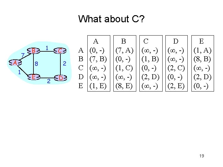
What is B’s update routing table after the exchange? 7 A B 1 2 8 1 E C 2 D A B C D E A (0, -) (7, B) (∞, -) (1, E) B (7, A) (0, -) (1, C) (∞, -) (8, E) C (∞, -) (1, B) (0, -) (2, D) (∞, -) D (∞, -) (2, C) (0, -) (2, E) E (1, A) (8, B) (∞, -) (2, D) (0, -) 18

Problems with DV Routing Link cost changes: good news travels fast – a new link will be known to all routers quickly. bad news travels slow “count to infinity” problem! A 1 B 1 C D 1 E 1 20

Count-to-Infinity Problem A 1 A B C D E B A (0, -) (1, B) (2, B) (3, B) (4, B) 1 B (1, A) (0, -) (1, C) (2, C) (3, C) C D 1 C (2, A) (1, B) (0, -) (1, D) (2, D) E 1 D (3, C) (2, C) (1, C) (0, -) (1, E) E (4, D) (3, D) (2, D) (1, D) (0, -) 21

Count-to-Infinity Problem A 1 B Let us look at A’s reachability, here is what we want: Distance vector will get this: 1 C D 1 E 1 A B (∞, -) C (∞, -) D (∞, -) E (∞, -) A B C D E B (∞, -) (0, -) (1, C) (2, C) (3, C) C (2, B) (1, B) (0, -) (1, D) (2, D) D (3, C) (2, C) (1, C) (0, -) (1, E) E (4, D) (3, D) (2, D) (1, D) (0, -) 22

Count-to-Infinity Problem A 1 B Let us look at A’s reachability C 1 D 1 E 1 B A (∞, -) C (2, B) D (3, C) E (4, D) Step 1 B A (3, C) C (4, D) D (3, C) E (4, D) Step 2 A B (5, C) C (4, B) D (5, C) E (4, D) A B (5, C) C (6, B) D (5, C) E (6, D) Step 3 23

Count-to-Infinity Problem A 1 B 1 C D 1 E 1 Step 3 B A (5, C) C (6, B) D (5, C) E (6, D) Step 4 B A (7, C) C (6, B) D (7, C) E (6, D) When can we reach the correct state? B A (∞, -) C (∞, -) D (∞, -) E (∞, -) 24

Fixes to Count-to-Infinity Problem • Split horizon – A router never advertises the cost of a destination to a neighbor if this neighbor is the next hop to that destination 25

Link State vs Distance Vector • Tells everyone about neighbors • Controlled flooding to exchange link state • Dijkstra’s algorithm • Each router computes its own table • May have oscillations • Open Shortest Path First (OSPF) • Tells neighbors about everyone • Exchanges distance vectors with neighbors • Bellman-Ford algorithm • Each router’s table is used by others • May have routing loops • Routing Information Protocol (RIP) 26