Chapter 5 Mining Frequent Patterns Association and Correlations

Chapter 5: Mining Frequent Patterns, Association and Correlations

What Is Frequent Pattern Analysis? • Frequent pattern: a pattern (a set of items, subsequences, substructures, etc. ) that occurs frequently in a data set • First proposed by Agrawal, Imielinski, and Swami [AIS 93] in the context of frequent itemsets and association rule mining • Motivation: Finding inherent regularities in data – What products were often purchased together? — Beer and diapers? ! – What are the subsequent purchases after buying a PC? – What kinds of DNA are sensitive to this new drug? – Can we automatically classify web documents? • Applications – Basket data analysis, cross-marketing, catalog design, sale campaign analysis, Web log (click stream) analysis, and DNA sequence analysis.

Why Is Freq. Pattern Mining Important? • Discloses an intrinsic and important property of data sets • Forms the foundation for many essential data mining tasks – Association, correlation, and causality analysis – Sequential, structural (e. g. , sub-graph) patterns – Pattern analysis in spatiotemporal, multimedia, timeseries, and stream data – Classification: associative classification – Cluster analysis: frequent pattern-based clustering – Data warehousing: iceberg cube and cube-gradient – Semantic data compression: fascicles – Broad applications

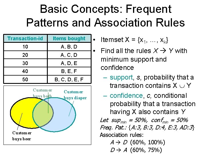
Basic Concepts: Frequent Patterns and Association Rules Transaction-id Items bought 10 A, B, D 20 A, C, D 30 A, D, E 40 B, E, F 50 B, C, D, E, F Customer buys both Customer buys beer Customer buys diaper • Itemset X = {x 1, …, xk} • Find all the rules X Y with minimum support and confidence – support, s, probability that a transaction contains X Y – confidence, c, conditional probability that a transaction having X also contains Y Let supmin = 50%, confmin = 50% Freq. Pat. : {A: 3, B: 3, D: 4, E: 3, AD: 3} Association rules: A D (60%, 100%) D A (60%, 75%)

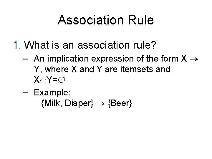
Association Rule 1. What is an association rule? – An implication expression of the form X Y, where X and Y are itemsets and X Y= – Example: {Milk, Diaper} {Beer}

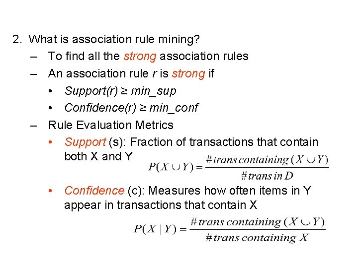
2. What is association rule mining? – To find all the strong association rules – An association rule r is strong if • Support(r) ≥ min_sup • Confidence(r) ≥ min_conf – Rule Evaluation Metrics • Support (s): Fraction of transactions that contain both X and Y • Confidence (c): Measures how often items in Y appear in transactions that contain X

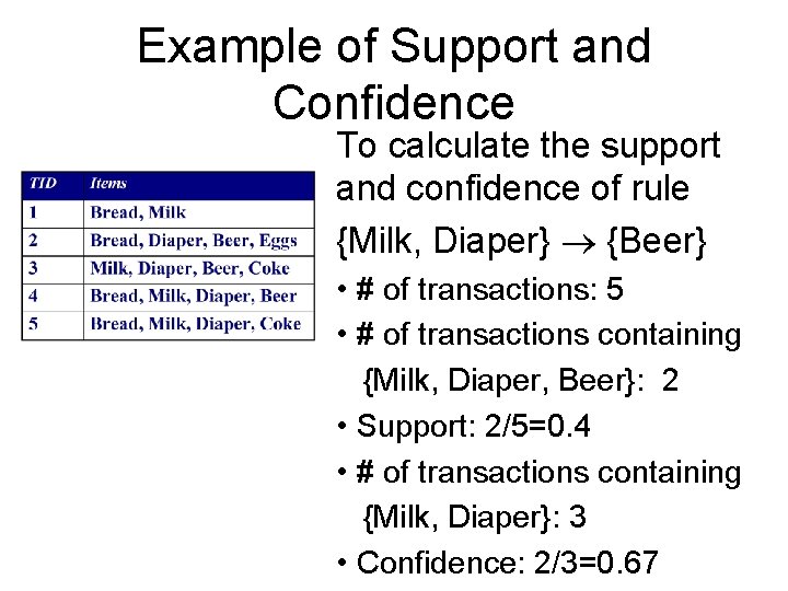
Example of Support and Confidence To calculate the support and confidence of rule {Milk, Diaper} {Beer} • # of transactions: 5 • # of transactions containing {Milk, Diaper, Beer}: 2 • Support: 2/5=0. 4 • # of transactions containing {Milk, Diaper}: 3 • Confidence: 2/3=0. 67

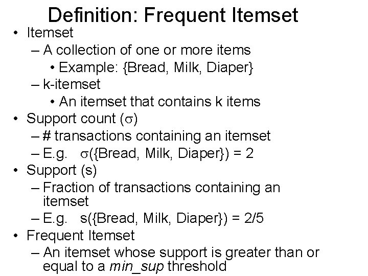
Definition: Frequent Itemset • Itemset – A collection of one or more items • Example: {Bread, Milk, Diaper} – k-itemset • An itemset that contains k items • Support count ( ) – # transactions containing an itemset – E. g. ({Bread, Milk, Diaper}) = 2 • Support (s) – Fraction of transactions containing an itemset – E. g. s({Bread, Milk, Diaper}) = 2/5 • Frequent Itemset – An itemset whose support is greater than or equal to a min_sup threshold

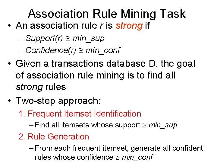
Association Rule Mining Task • An association rule r is strong if – Support(r) ≥ min_sup – Confidence(r) ≥ min_conf • Given a transactions database D, the goal of association rule mining is to find all strong rules • Two-step approach: 1. Frequent Itemset Identification – Find all itemsets whose support min_sup 2. Rule Generation – From each frequent itemset, generate all confident rules whose confidence min_conf

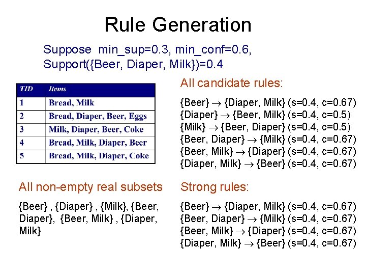
Rule Generation Suppose min_sup=0. 3, min_conf=0. 6, Support({Beer, Diaper, Milk})=0. 4 All candidate rules: {Beer} {Diaper, Milk} (s=0. 4, c=0. 67) {Diaper} {Beer, Milk} (s=0. 4, c=0. 5) {Milk} {Beer, Diaper} (s=0. 4, c=0. 5) {Beer, Diaper} {Milk} (s=0. 4, c=0. 67) {Beer, Milk} {Diaper} (s=0. 4, c=0. 67) {Diaper, Milk} {Beer} (s=0. 4, c=0. 67) All non-empty real subsets Strong rules: {Beer} , {Diaper} , {Milk}, {Beer, Diaper}, {Beer, Milk} , {Diaper, Milk} {Beer} {Diaper, Milk} (s=0. 4, c=0. 67) {Beer, Diaper} {Milk} (s=0. 4, c=0. 67) {Beer, Milk} {Diaper} (s=0. 4, c=0. 67) {Diaper, Milk} {Beer} (s=0. 4, c=0. 67)

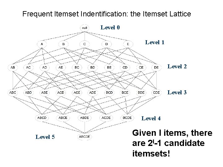
Frequent Itemset Indentification: the Itemset Lattice Level 0 Level 1 Level 2 Level 3 Level 4 Level 5 Given I items, there are 2 I-1 candidate itemsets!

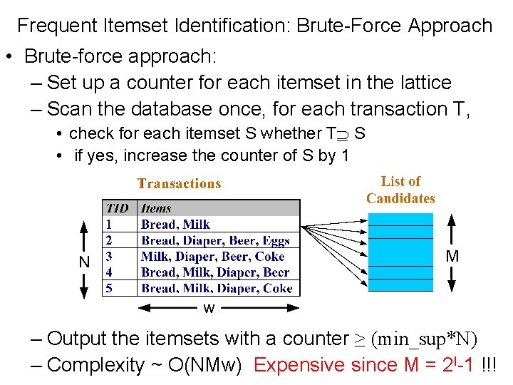
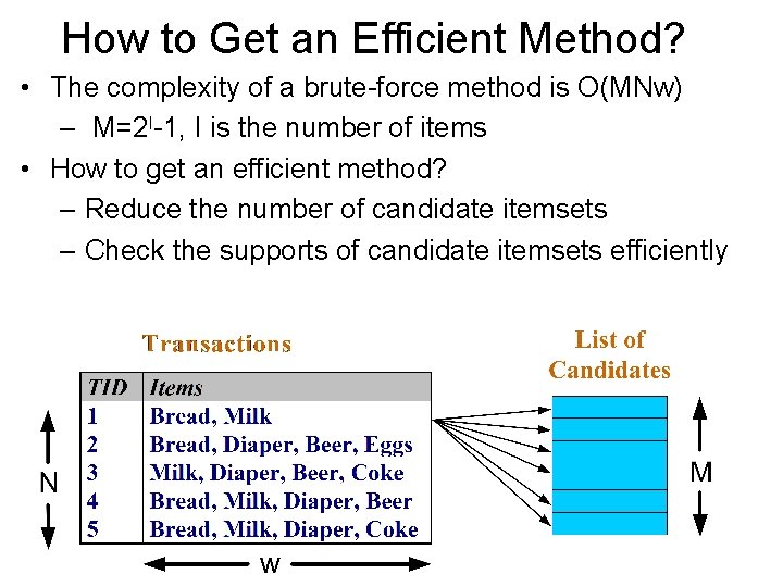
Frequent Itemset Identification: Brute-Force Approach • Brute-force approach: – Set up a counter for each itemset in the lattice – Scan the database once, for each transaction T, • check for each itemset S whether T S • if yes, increase the counter of S by 1 – Output the itemsets with a counter ≥ (min_sup*N) – Complexity ~ O(NMw) Expensive since M = 2 I-1 !!!

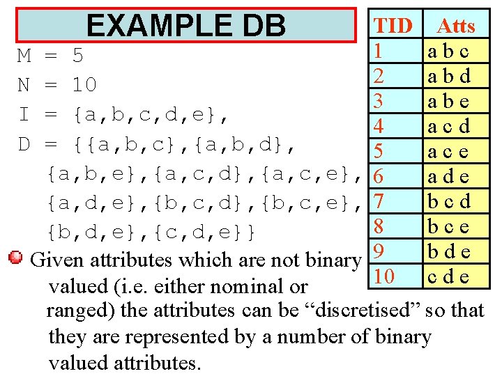
EXAMPLE DB TID Atts 1 abc M = 5 2 abd N = 10 3 abe I = {a, b, c, d, e}, 4 acd D = {{a, b, c}, {a, b, d}, 5 ace {a, b, e}, {a, c, d}, {a, c, e}, 6 ade bcd {a, d, e}, {b, c, d}, {b, c, e}, 7 8 bce {b, d, e}, {c, d, e}} bde Given attributes which are not binary 9 10 c d e valued (i. e. either nominal or ranged) the attributes can be “discretised” so that they are represented by a number of binary valued attributes.

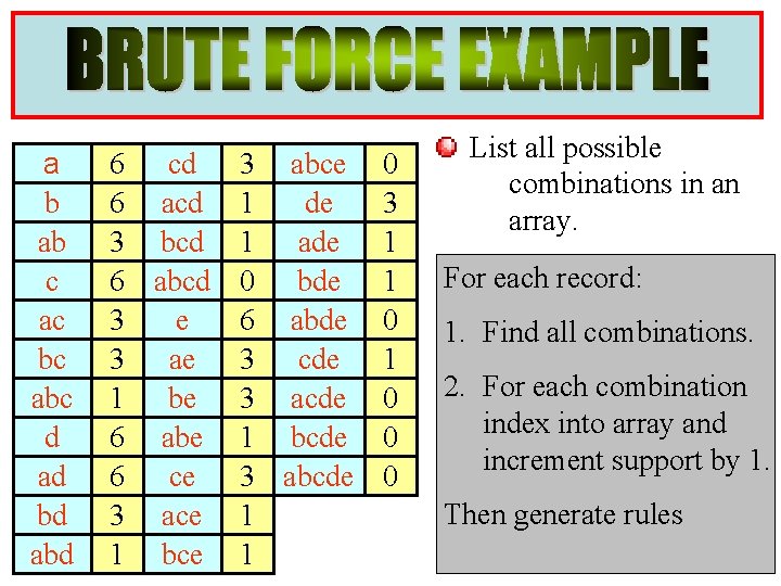
a b ab c ac bc abc d ad bd abd 6 cd 3 abce 6 acd 1 de 3 bcd 1 ade 6 abcd 0 bde 3 e 6 abde 3 ae 3 cde 1 be 3 acde 6 abe 1 bcde 6 ce 3 abcde 3 ace 1 1 bce 1 0 3 1 1 0 0 0 List all possible combinations in an array. For each record: 1. Find all combinations. 2. For each combination index into array and increment support by 1. Then generate rules

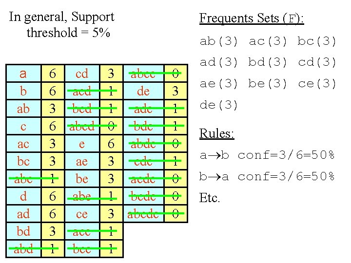
In general, Support threshold = 5% a b ab c ac bc abc d ad bd abd 6 cd 3 abce 6 acd 1 de 3 bcd 1 ade 6 abcd 0 bde 3 e 6 abde 3 ae 3 cde 1 be 3 acde 6 abe 1 bcde 6 ce 3 abcde 3 ace 1 1 bce 1 Frequents Sets (F): ab(3) ac(3) bc(3) 0 3 1 1 0 0 0 ad(3) bd(3) cd(3) ae(3) be(3) ce(3) de(3) Rules: a b conf=3/6=50% b a conf=3/6=50% Etc.

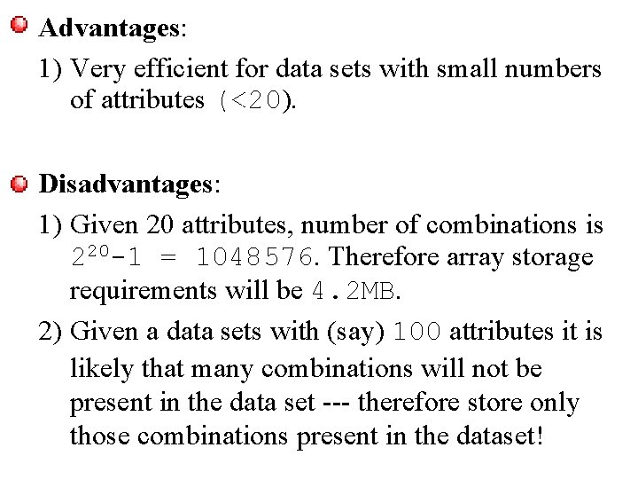
Advantages: 1) Very efficient for data sets with small numbers of attributes (<20). Disadvantages: 1) Given 20 attributes, number of combinations is 220 -1 = 1048576. Therefore array storage requirements will be 4. 2 MB. 2) Given a data sets with (say) 100 attributes it is likely that many combinations will not be present in the data set --- therefore store only those combinations present in the dataset!

How to Get an Efficient Method? • The complexity of a brute-force method is O(MNw) – M=2 I-1, I is the number of items • How to get an efficient method? – Reduce the number of candidate itemsets – Check the supports of candidate itemsets efficiently

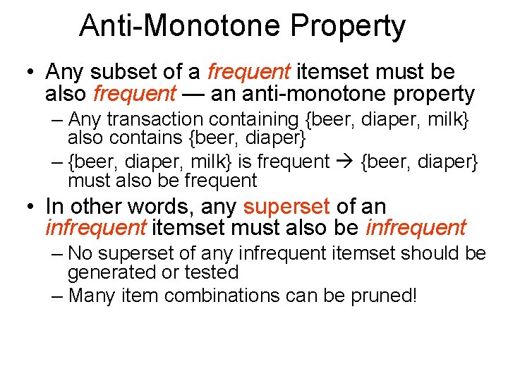
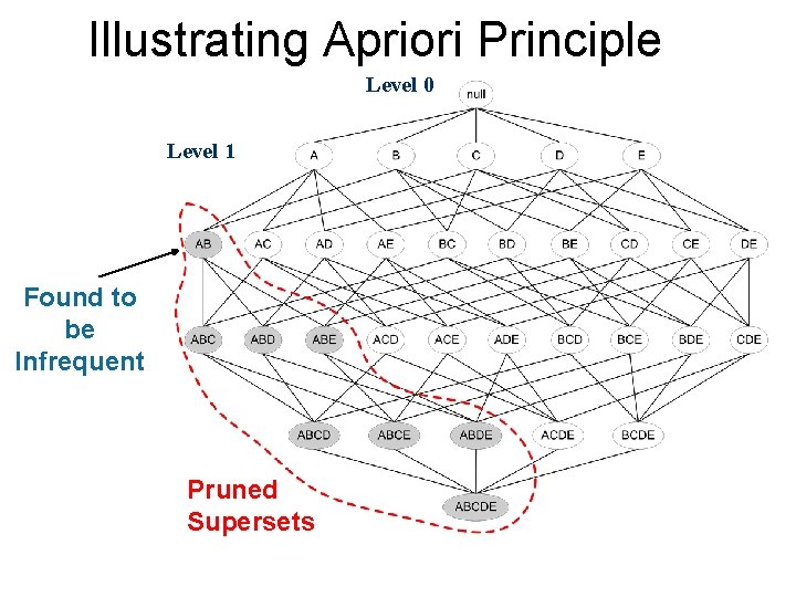
Anti-Monotone Property • Any subset of a frequent itemset must be also frequent — an anti-monotone property – Any transaction containing {beer, diaper, milk} also contains {beer, diaper} – {beer, diaper, milk} is frequent {beer, diaper} must also be frequent • In other words, any superset of an infrequent itemset must also be infrequent – No superset of any infrequent itemset should be generated or tested – Many item combinations can be pruned!

Illustrating Apriori Principle Level 0 Level 1 Found to be Infrequent Pruned Supersets

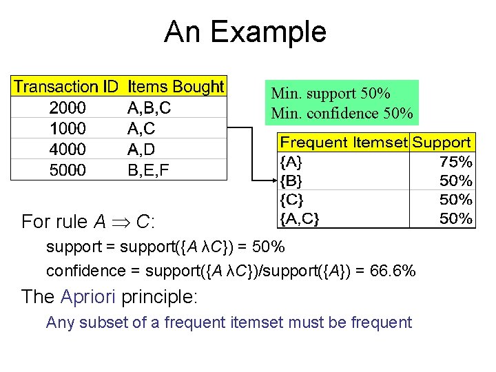
An Example Min. support 50% Min. confidence 50% For rule A C: support = support({A λC}) = 50% confidence = support({A λC})/support({A}) = 66. 6% The Apriori principle: Any subset of a frequent itemset must be frequent

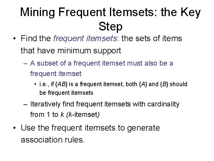
Mining Frequent Itemsets: the Key Step • Find the frequent itemsets: the sets of items that have minimum support – A subset of a frequent itemset must also be a frequent itemset • i. e. , if {AB} is a frequent itemset, both {A} and {B} should be frequent itemsets – Iteratively find frequent itemsets with cardinality from 1 to k (k-itemset) • Use the frequent itemsets to generate association rules.

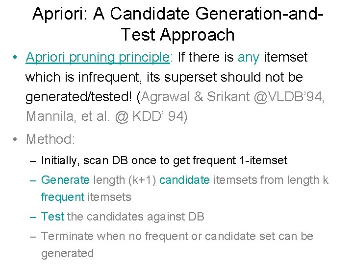
Apriori: A Candidate Generation-and. Test Approach • Apriori pruning principle: If there is any itemset which is infrequent, its superset should not be generated/tested! (Agrawal & Srikant @VLDB’ 94, Mannila, et al. @ KDD’ 94) • Method: – Initially, scan DB once to get frequent 1 -itemset – Generate length (k+1) candidate itemsets from length k frequent itemsets – Test the candidates against DB – Terminate when no frequent or candidate set can be generated

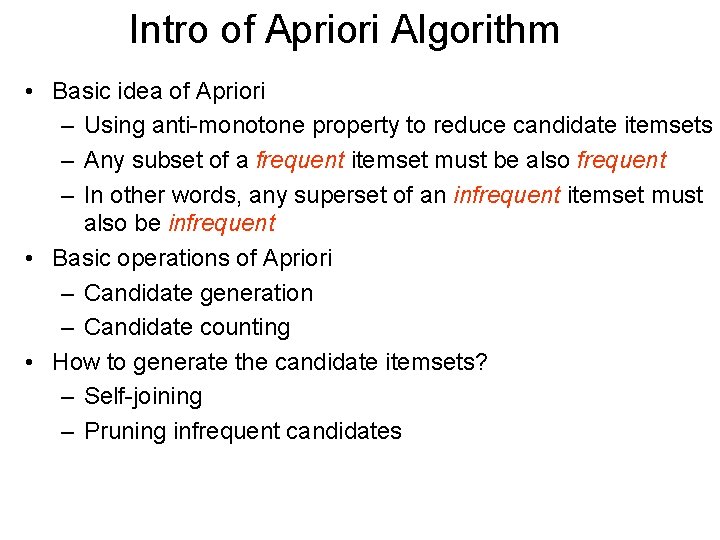
Intro of Apriori Algorithm • Basic idea of Apriori – Using anti-monotone property to reduce candidate itemsets – Any subset of a frequent itemset must be also frequent – In other words, any superset of an infrequent itemset must also be infrequent • Basic operations of Apriori – Candidate generation – Candidate counting • How to generate the candidate itemsets? – Self-joining – Pruning infrequent candidates

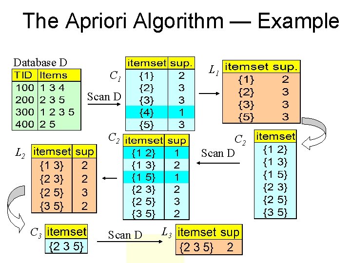
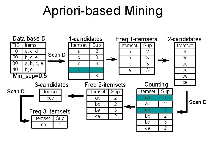
The Apriori Algorithm — Example Database D L 1 C 1 Scan D C 2 Scan D L 2 C 3 Scan D L 3

Apriori-based Mining Data base D TID 10 20 30 40 Items a, c, d b, c, e a, b, c, e b, e 1 -candidates Scan D Min_sup=0. 5 3 -candidates Scan D Itemset bce Freq 3 -itemsets Itemset bce Sup 2 Itemset a b c d e Sup 2 3 3 1 3 Freq 1 -itemsets Itemset a b c e Freq 2 -itemsets Itemset ac bc be ce Sup 2 2 3 2 2 -candidates Sup 2 3 3 3 Counting Itemset ab ac ae bc be ce Sup 1 2 3 2 Itemset ab ac ae bc be ce Scan D

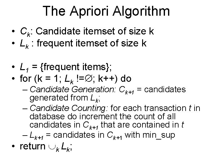
The Apriori Algorithm • Ck: Candidate itemset of size k • Lk : frequent itemset of size k • L 1 = {frequent items}; • for (k = 1; Lk != ; k++) do – Candidate Generation: Ck+1 = candidates generated from Lk; – Candidate Counting: for each transaction t in database do increment the count of all candidates in Ck+1 that are contained in t – Lk+1 = candidates in Ck+1 with min_sup • return k Lk;

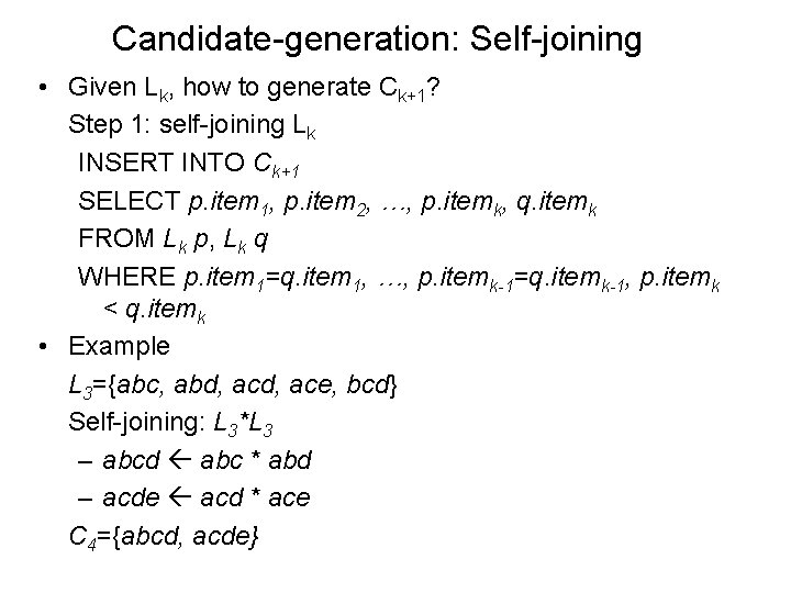
Candidate-generation: Self-joining • Given Lk, how to generate Ck+1? Step 1: self-joining Lk INSERT INTO Ck+1 SELECT p. item 1, p. item 2, …, p. itemk, q. itemk FROM Lk p, Lk q WHERE p. item 1=q. item 1, …, p. itemk-1=q. itemk-1, p. itemk < q. itemk • Example L 3={abc, abd, ace, bcd} Self-joining: L 3*L 3 – abcd abc * abd – acde acd * ace C 4={abcd, acde}

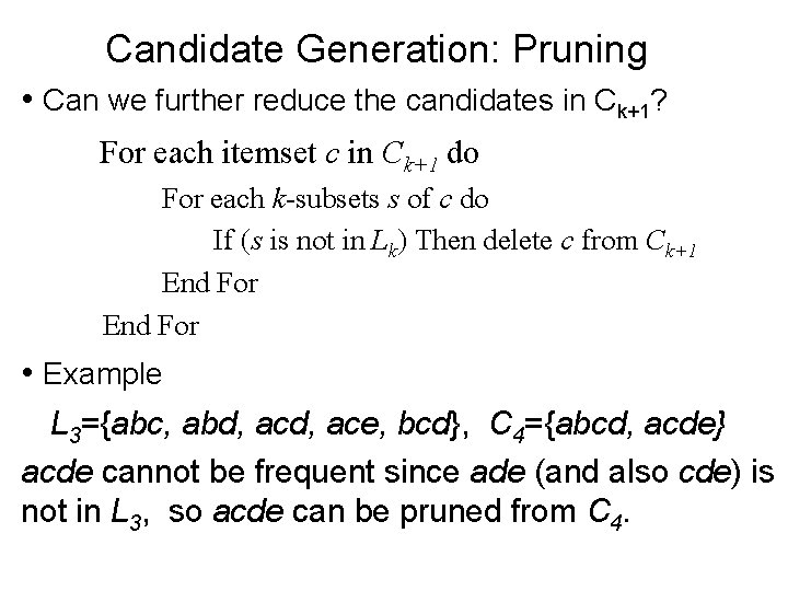
Candidate Generation: Pruning • Can we further reduce the candidates in Ck+1? For each itemset c in Ck+1 do For each k-subsets s of c do If (s is not in Lk) Then delete c from Ck+1 End For • Example L 3={abc, abd, ace, bcd}, C 4={abcd, acde} acde cannot be frequent since ade (and also cde) is not in L 3, so acde can be pruned from C 4.

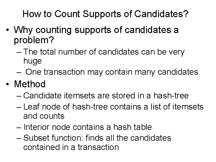
How to Count Supports of Candidates? • Why counting supports of candidates a problem? – The total number of candidates can be very huge – One transaction may contain many candidates • Method – Candidate itemsets are stored in a hash-tree – Leaf node of hash-tree contains a list of itemsets and counts – Interior node contains a hash table – Subset function: finds all the candidates contained in a transaction

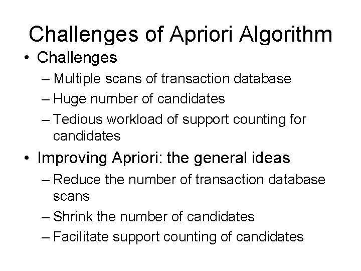
Challenges of Apriori Algorithm • Challenges • Improving Apriori: the general ideas – Multiple scans of transaction database –– Reduce the number of transaction database Huge number of candidates – scans Tedious workload of support counting for • DIC: Start count k-itemset as early as possible candidates • • S. Brin R. Motwani, J. Ullman, and S. Tsur, Improving Apriori: the general ideas SIGMOD’ 97. Reducethe thenumberofofcandidates transaction database –– Shrink scans • DHP: A k-itemset whose corresponding hashing bucket count is below the threshold cannot be frequent – Shrink the number of candidates • J. Park, M. Chen, and P. Yu, SIGMOD’ 95 – Facilitate support counting of candidates

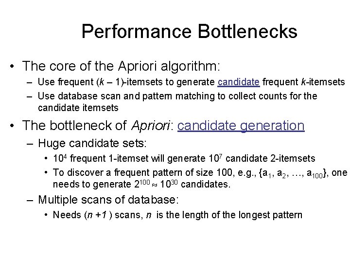
Performance Bottlenecks • The core of the Apriori algorithm: – Use frequent (k – 1)-itemsets to generate candidate frequent k-itemsets – Use database scan and pattern matching to collect counts for the candidate itemsets • The bottleneck of Apriori: candidate generation – Huge candidate sets: • 104 frequent 1 -itemset will generate 107 candidate 2 -itemsets • To discover a frequent pattern of size 100, e. g. , {a 1, a 2, …, a 100}, one needs to generate 2100 1030 candidates. – Multiple scans of database: • Needs (n +1 ) scans, n is the length of the longest pattern