Chapter 5 LOGARITHMIC FUNCTIONS Section 5 1 Logarithms

Chapter 5 LOGARITHMIC FUNCTIONS Section 5. 1 Logarithms and Their Properties Section 5. 2 Logarithms and Exponential Models Section 5. 3 The Logarithmic Function and Its Applications Section 5. 4 Logarithmic Scales Functions Modeling Change: A Preparation for Calculus, 5 th Edition, 2014, Connally 1

5. 1 LOGARITHMS AND THEIR PROPERTIES Functions Modeling Change: A Preparation for Calculus, 5 th Edition, 2014, Connally 2

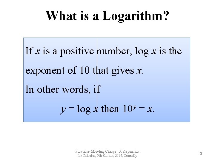
What is a Logarithm? If x is a positive number, log x is the exponent of 10 that gives x. In other words, if y = log x then 10 y = x. Functions Modeling Change: A Preparation for Calculus, 5 th Edition, 2014, Connally 3

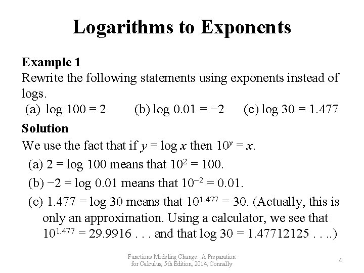
Logarithms to Exponents Example 1 Rewrite the following statements using exponents instead of logs. (a) log 100 = 2 (b) log 0. 01 = − 2 (c) log 30 = 1. 477 Solution We use the fact that if y = log x then 10 y = x. (a) 2 = log 100 means that 102 = 100. (b) − 2 = log 0. 01 means that 10− 2 = 0. 01. (c) 1. 477 = log 30 means that 101. 477 = 30. (Actually, this is only an approximation. Using a calculator, we see that 101. 477 = 29. 9916. . . and that log 30 = 1. 47712125. . ) Functions Modeling Change: A Preparation for Calculus, 5 th Edition, 2014, Connally 4

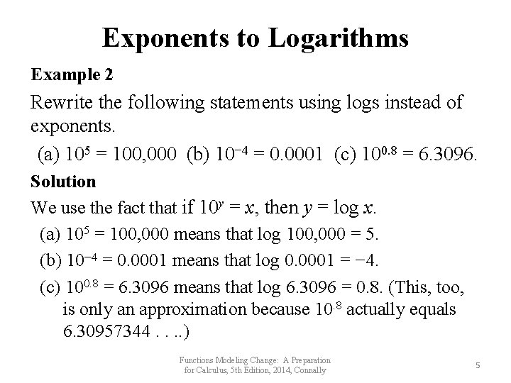
Exponents to Logarithms Example 2 Rewrite the following statements using logs instead of exponents. (a) 105 = 100, 000 (b) 10− 4 = 0. 0001 (c) 100. 8 = 6. 3096. Solution We use the fact that if 10 y = x, then y = log x. (a) 105 = 100, 000 means that log 100, 000 = 5. (b) 10− 4 = 0. 0001 means that log 0. 0001 = − 4. (c) 100. 8 = 6. 3096 means that log 6. 3096 = 0. 8. (This, too, is only an approximation because 10. 8 actually equals 6. 30957344. . ) Functions Modeling Change: A Preparation for Calculus, 5 th Edition, 2014, Connally 5

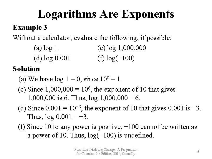
Logarithms Are Exponents Example 3 Without a calculator, evaluate the following, if possible: (a) log 1 (c) log 1, 000 (d) log 0. 001 (f) log(− 100) Solution (a) We have log 1 = 0, since 100 = 1. (c) Since 1, 000 = 106, the exponent of 10 that gives 1, 000 is 6. Thus, log 1, 000 = 6. (d) Since 0. 001 = 10− 3, the exponent of 10 that gives 0. 001 is − 3. Thus, log 0. 001 = − 3. (f) Since 10 to any power is positive, − 100 cannot be written as a power of 10. Thus, log(− 100) is undefined. Functions Modeling Change: A Preparation for Calculus, 5 th Edition, 2014, Connally 6

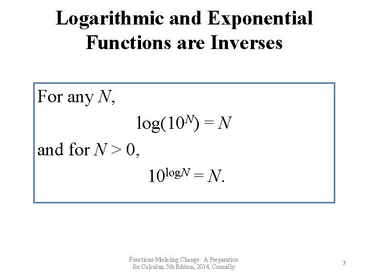
Logarithmic and Exponential Functions are Inverses For any N, log(10 N) = N and for N > 0, 10 log. N = N. Functions Modeling Change: A Preparation for Calculus, 5 th Edition, 2014, Connally 7

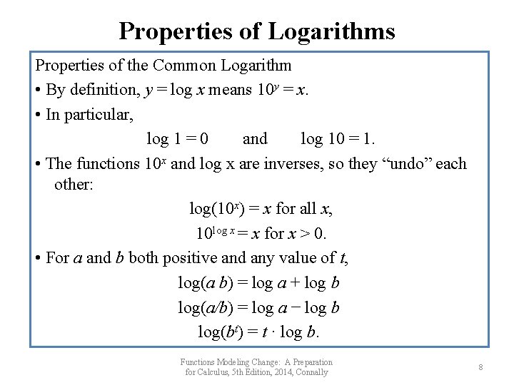
Properties of Logarithms Properties of the Common Logarithm • By definition, y = log x means 10 y = x. • In particular, log 1 = 0 and log 10 = 1. • The functions 10 x and log x are inverses, so they “undo” each other: log(10 x) = x for all x, 10 log x = x for x > 0. • For a and b both positive and any value of t, log(a b) = log a + log b log(a/b) = log a − log b log(bt) = t · log b. Functions Modeling Change: A Preparation for Calculus, 5 th Edition, 2014, Connally 8

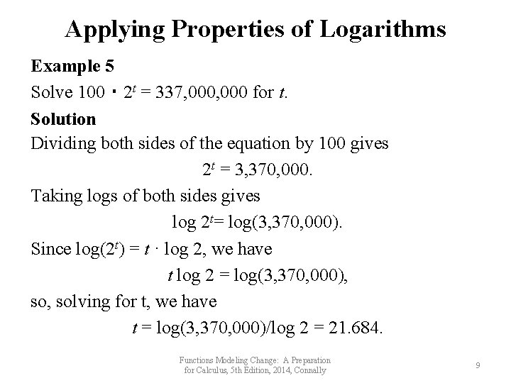
Applying Properties of Logarithms Example 5 Solve 100・ 2 t = 337, 000 for t. Solution Dividing both sides of the equation by 100 gives 2 t = 3, 370, 000. Taking logs of both sides gives log 2 t= log(3, 370, 000). Since log(2 t) = t · log 2, we have t log 2 = log(3, 370, 000), solving for t, we have t = log(3, 370, 000)/log 2 = 21. 684. Functions Modeling Change: A Preparation for Calculus, 5 th Edition, 2014, Connally 9

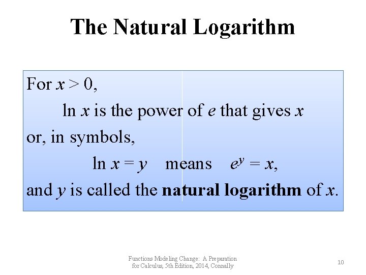
The Natural Logarithm For x > 0, ln x is the power of e that gives x or, in symbols, ln x = y means ey = x, and y is called the natural logarithm of x. Functions Modeling Change: A Preparation for Calculus, 5 th Edition, 2014, Connally 10

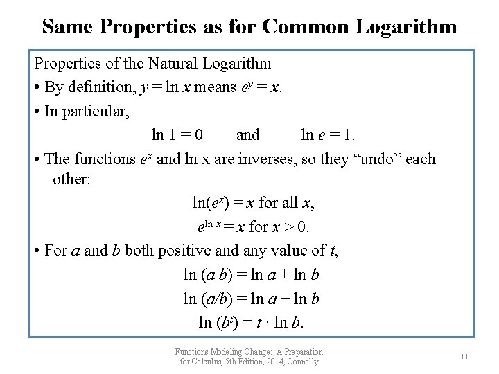
Same Properties as for Common Logarithm Properties of the Natural Logarithm • By definition, y = ln x means ey = x. • In particular, ln 1 = 0 and ln e = 1. • The functions ex and ln x are inverses, so they “undo” each other: ln(ex) = x for all x, eln x = x for x > 0. • For a and b both positive and any value of t, ln (a b) = ln a + ln b ln (a/b) = ln a − ln b ln (bt) = t · ln b. Functions Modeling Change: A Preparation for Calculus, 5 th Edition, 2014, Connally 11

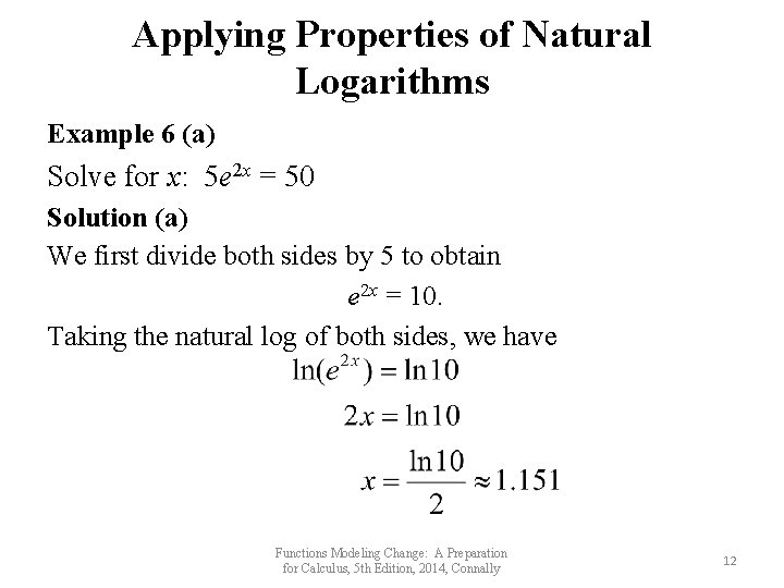
Applying Properties of Natural Logarithms Example 6 (a) Solve for x: 5 e 2 x = 50 Solution (a) We first divide both sides by 5 to obtain e 2 x = 10. Taking the natural log of both sides, we have Functions Modeling Change: A Preparation for Calculus, 5 th Edition, 2014, Connally 12

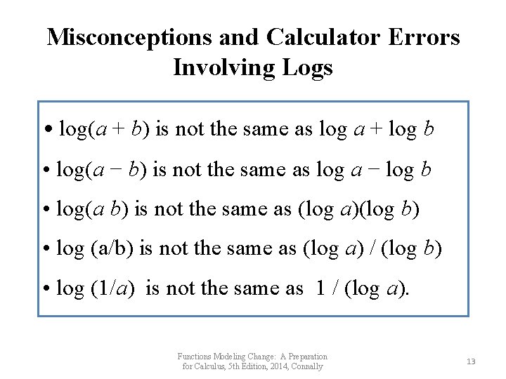
Misconceptions and Calculator Errors Involving Logs • log(a + b) is not the same as log a + log b • log(a − b) is not the same as log a − log b • log(a b) is not the same as (log a)(log b) • log (a/b) is not the same as (log a) / (log b) • log (1/a) is not the same as 1 / (log a). Functions Modeling Change: A Preparation for Calculus, 5 th Edition, 2014, Connally 13

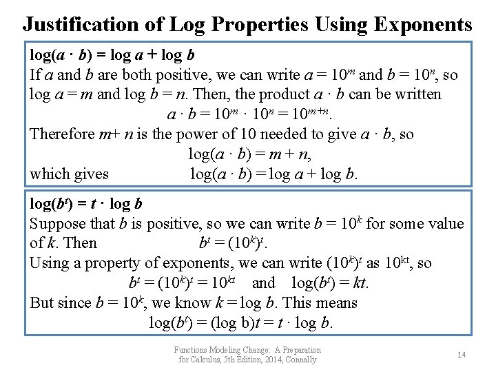
Justification of Log Properties Using Exponents log(a · b) = log a + log b If a and b are both positive, we can write a = 10 m and b = 10 n, so log a = m and log b = n. Then, the product a · b can be written a · b = 10 m · 10 n = 10 m+n. Therefore m+ n is the power of 10 needed to give a · b, so log(a · b) = m + n, which gives log(a · b) = log a + log b. log(bt) = t · log b Suppose that b is positive, so we can write b = 10 k for some value of k. Then bt = (10 k)t. Using a property of exponents, we can write (10 k)t as 10 kt, so bt = (10 k)t = 10 kt and log(bt) = kt. But since b = 10 k, we know k = log b. This means log(bt) = (log b)t = t · log b. Functions Modeling Change: A Preparation for Calculus, 5 th Edition, 2014, Connally 14

5. 2 LOGARITHMS AND EXPONENTIAL MODELS Functions Modeling Change: A Preparation for Calculus, 5 th Edition, 2014, Connally 15

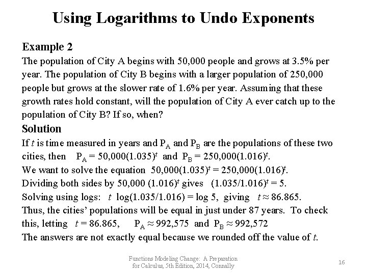
Using Logarithms to Undo Exponents Example 2 The population of City A begins with 50, 000 people and grows at 3. 5% per year. The population of City B begins with a larger population of 250, 000 people but grows at the slower rate of 1. 6% per year. Assuming that these growth rates hold constant, will the population of City A ever catch up to the population of City B? If so, when? Solution If t is time measured in years and PA and PB are the populations of these two cities, then PA = 50, 000(1. 035)t and PB = 250, 000(1. 016)t. We want to solve the equation 50, 000(1. 035)t = 250, 000(1. 016)t. Dividing both sides by 50, 000 (1. 016)t gives (1. 035/1. 016)t = 5. Solving using logs: t log(1. 035/1. 016) = log 5, giving t ≈ 86. 865. Thus, the cities’ populations will be equal in just under 87 years. To check this, letting t = 86. 865, PA ≈ 992, 575 and PB ≈ 992, 572 The answers are not exactly equal because we rounded off the value of t. Functions Modeling Change: A Preparation for Calculus, 5 th Edition, 2014, Connally 16

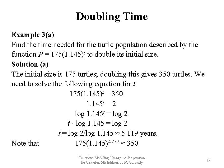
Doubling Time Example 3(a) Find the time needed for the turtle population described by the function P = 175(1. 145)t to double its initial size. Solution (a) The initial size is 175 turtles; doubling this gives 350 turtles. We need to solve the following equation for t: 175(1. 145)t = 350 1. 145 t = 2 log 1. 145 t = log 2 t · log 1. 145 = log 2 t = log 2/log 1. 145 ≈ 5. 119 years. Note that 175(1. 145)5. 119 ≈ 350 Functions Modeling Change: A Preparation for Calculus, 5 th Edition, 2014, Connally 17

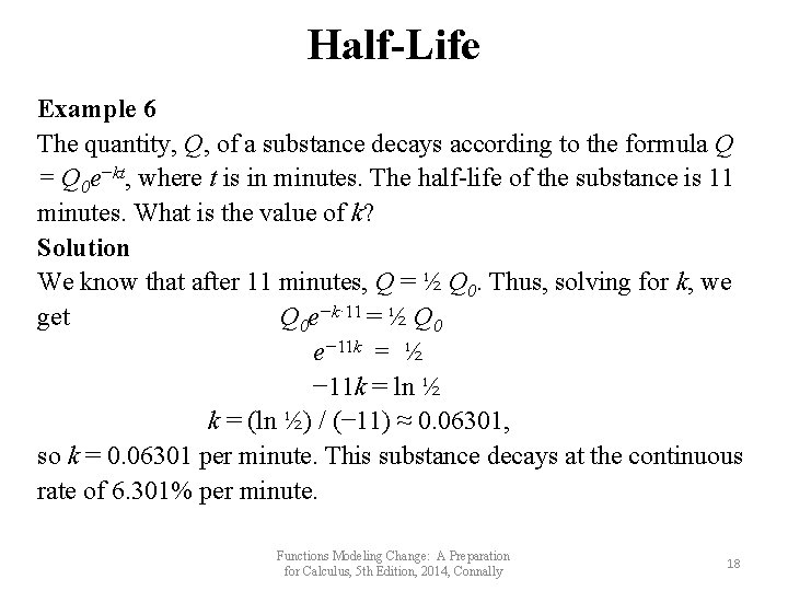
Half-Life Example 6 The quantity, Q, of a substance decays according to the formula Q = Q 0 e−kt, where t is in minutes. The half-life of the substance is 11 minutes. What is the value of k? Solution We know that after 11 minutes, Q = ½ Q 0. Thus, solving for k, we get Q 0 e−k· 11 = ½ Q 0 e− 11 k = ½ − 11 k = ln ½ k = (ln ½) / (− 11) ≈ 0. 06301, so k = 0. 06301 per minute. This substance decays at the continuous rate of 6. 301% per minute. Functions Modeling Change: A Preparation for Calculus, 5 th Edition, 2014, Connally 18

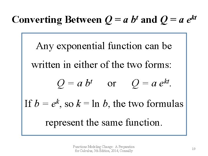
Converting Between Q = a bt and Q = a ekt Any exponential function can be written in either of the two forms: Q = a bt or Q = a ekt. If b = ek, so k = ln b, the two formulas represent the same function. Functions Modeling Change: A Preparation for Calculus, 5 th Edition, 2014, Connally 19

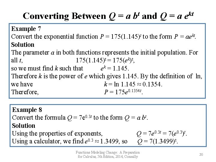
Converting Between Q = a bt and Q = a ekt Example 7 Convert the exponential function P = 175(1. 145)t to the form P = aekt. Solution The parameter a in both functions represents the initial population. For all t, 175(1. 145)t = 175(ek)t, so we must find k such that ek = 1. 145. Therefore k is the power of e which gives 1. 145. By the definition of ln, we have k = ln 1. 145 ≈ 0. 1354. Therefore, P = 175 e 0. 1354 t. Example 8 Convert the formula Q = 7 e 0. 3 t to the form Q = a bt. Solution Using the properties of exponents, Q = 7 e 0. 3 t = 7(e 0. 3)t. Using a calculator, we find e 0. 3 ≈ 1. 3499, so Q = 7(1. 3499)t. Functions Modeling Change: A Preparation for Calculus, 5 th Edition, 2014, Connally 20

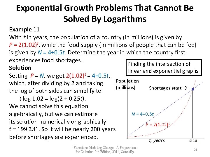
Exponential Growth Problems That Cannot Be Solved By Logarithms Example 11 With t in years, the population of a country (in millions) is given by P = 2(1. 02)t, while the food supply (in millions of people that can be fed) is given by N = 4+0. 5 t. Determine the year in which the country first experiences food shortages. Finding the intersection of Solution linear and exponential graphs t Setting P = N, we get 2(1. 02) = 4+0. 5 t, Population which, after dividing by 2 and taking (millions) Shortages start → the log of both sides can simplify to t log 1. 02 = log(2 + 0. 25 t). We cannot solve this equation N = 4+0. 5 t algebraically, but we can estimate its solution numerically or graphically: P = 2(1. 02)t t ≈ 199. 381. So it will be nearly 200 years before shortages are experienced. t, years Functions Modeling Change: A Preparation for Calculus, 5 th Edition, 2014, Connally 21

5. 3 THE LOGARITHMIC FUNCTION AND ITS APPLICATIONS Functions Modeling Change: A Preparation for Calculus, 5 th Edition, 2014, Connally 22

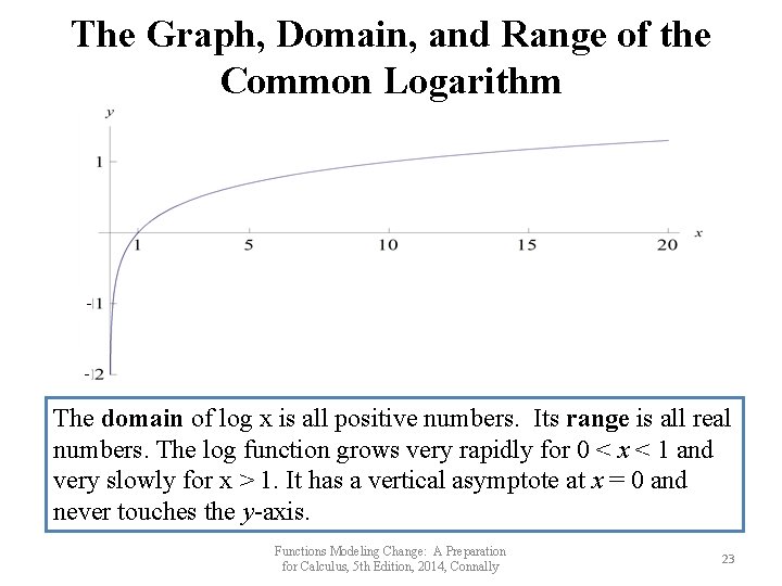
The Graph, Domain, and Range of the Common Logarithm - The domain of log x is all positive numbers. Its range is all real numbers. The log function grows very rapidly for 0 < x < 1 and very slowly for x > 1. It has a vertical asymptote at x = 0 and never touches the y-axis. Functions Modeling Change: A Preparation for Calculus, 5 th Edition, 2014, Connally 23

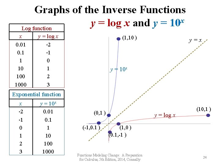
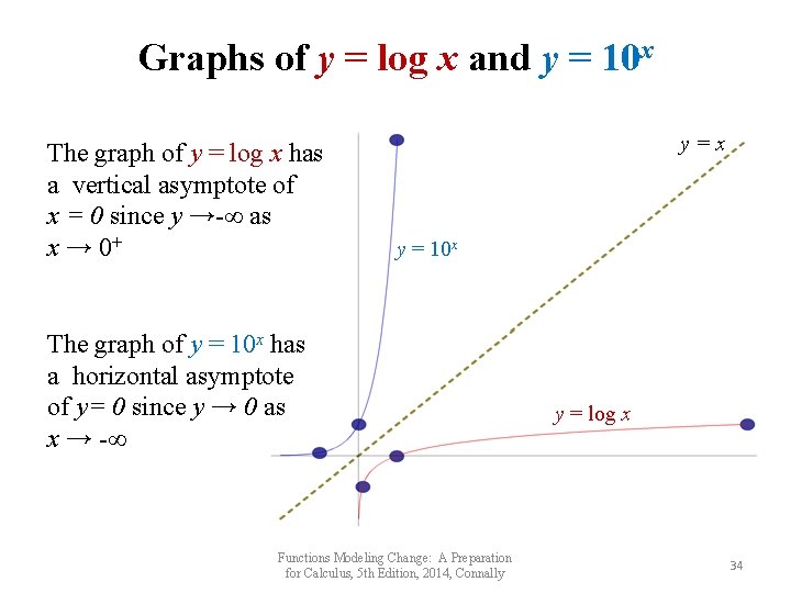
Graphs of the Inverse Functions x y = log x and y = 10 Log function x 0. 01 0. 1 1 10 1000 y = log x -2 -1 0 1 2 3 (1, 10 ) y=x y = 10 x Exponential function x -2 -1 0 1 2 3 y = 10 x 0. 01 0. 1 1 10 1000 (0, 1 ) (-1, 0. 1 ) y = log x (10, 1 ) (1, 0 ) (0. 1, -1 ) Functions Modeling Change: A Preparation for Calculus, 5 th Edition, 2014, Connally 24

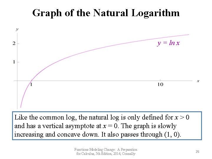
Graph of the Natural Logarithm y = ln x Like the common log, the natural log is only defined for x > 0 and has a vertical asymptote at x = 0. The graph is slowly increasing and concave down. It also passes through (1, 0). Functions Modeling Change: A Preparation for Calculus, 5 th Edition, 2014, Connally 25

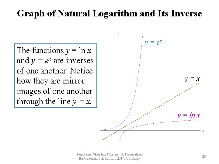
Graph of Natural Logarithm and Its Inverse The functions y = ln x and y = ex are inverses of one another. Notice how they are mirror images of one another through the line y = x. y = ex y=x y = ln x Functions Modeling Change: A Preparation for Calculus, 5 th Edition, 2014, Connally 26

Chemical Acidity In chemistry, the acidity of a liquid is expressed using p. H. The acidity depends on the hydrogen ion concentration in the liquid (in moles per liter); this concentration is written [H+]. The greater the hydrogen ion concentration, the more acidic the solution. The p. H is defined as: p. H = −log[H+]. Functions Modeling Change: A Preparation for Calculus, 5 th Edition, 2014, Connally 27

Chemical Acidity Example 2 The hydrogen ion concentration of seawater is [H+] = 1. 1 · 10− 8. Estimate the p. H of seawater. Then check your answer with a calculator. Solution • We want to estimate p. H = −log(1. 1 · 10− 8). • Since 1. 1 · 10− 8 ≈ 10− 8 and log 10− 8 = − 8, we know that p. H = −log(1. 1 · 10− 8) ≈ −(− 8) = 8. • Using a calculator, we have p. H = −log(1. 1 · 10− 8) = 7. 959. Functions Modeling Change: A Preparation for Calculus, 5 th Edition, 2014, Connally 28

Logarithms and Orders of Magnitude • Logarithms are useful in measuring quantities whose magnitudes vary widely, such as acidity (p. H), sound (decibels), and earthquakes (the Richter scale). • If one object is 10 times heavier than another, we say it is an order of magnitude heavier. If one quantity is two factors of 10 greater than another, we say it is two orders of magnitude greater. Functions Modeling Change: A Preparation for Calculus, 5 th Edition, 2014, Connally 29

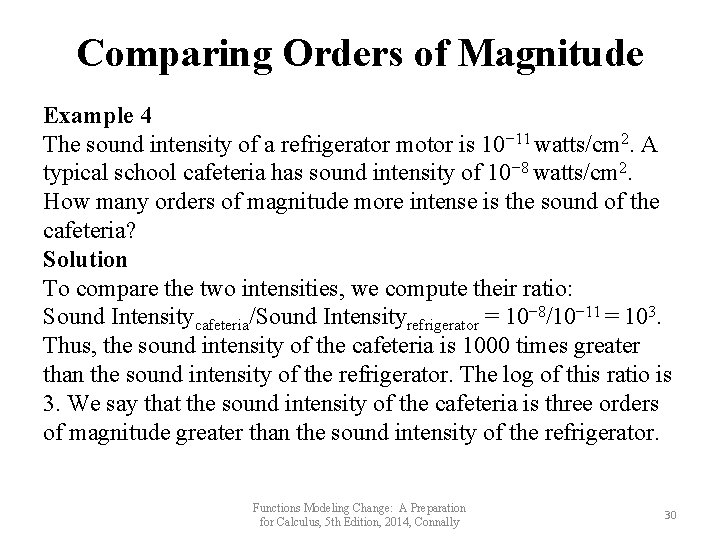
Comparing Orders of Magnitude Example 4 The sound intensity of a refrigerator motor is 10− 11 watts/cm 2. A typical school cafeteria has sound intensity of 10− 8 watts/cm 2. How many orders of magnitude more intense is the sound of the cafeteria? Solution To compare the two intensities, we compute their ratio: Sound Intensitycafeteria/Sound Intensityrefrigerator = 10− 8/10− 11 = 103. Thus, the sound intensity of the cafeteria is 1000 times greater than the sound intensity of the refrigerator. The log of this ratio is 3. We say that the sound intensity of the cafeteria is three orders of magnitude greater than the sound intensity of the refrigerator. Functions Modeling Change: A Preparation for Calculus, 5 th Edition, 2014, Connally 30

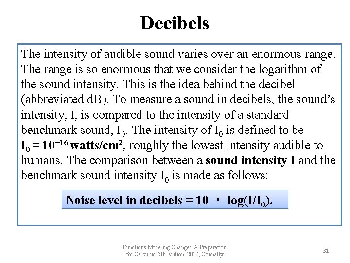
Decibels The intensity of audible sound varies over an enormous range. The range is so enormous that we consider the logarithm of the sound intensity. This is the idea behind the decibel (abbreviated d. B). To measure a sound in decibels, the sound’s intensity, I, is compared to the intensity of a standard benchmark sound, I 0. The intensity of I 0 is defined to be I 0 = 10− 16 watts/cm 2, roughly the lowest intensity audible to humans. The comparison between a sound intensity I and the benchmark sound intensity I 0 is made as follows: Noise level in decibels = 10 ・ log(I/I 0). Functions Modeling Change: A Preparation for Calculus, 5 th Edition, 2014, Connally 31

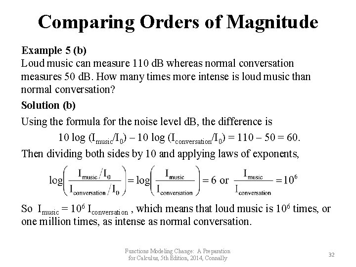
Comparing Orders of Magnitude Example 5 (b) Loud music can measure 110 d. B whereas normal conversation measures 50 d. B. How many times more intense is loud music than normal conversation? Solution (b) Using the formula for the noise level d. B, the difference is 10 log (Imusic/I 0) – 10 log (Iconversation/I 0) = 110 – 50 = 60. Then dividing both sides by 10 and applying laws of exponents, So Imusic = 106 Iconversation , which means that loud music is 106 times, or one million times, as intense as normal conversation. Functions Modeling Change: A Preparation for Calculus, 5 th Edition, 2014, Connally 32

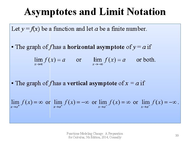
Asymptotes and Limit Notation Let y = f(x) be a function and let a be a finite number. • The graph of f has a horizontal asymptote of y = a if • The graph of f has a vertical asymptote of x = a if Functions Modeling Change: A Preparation for Calculus, 5 th Edition, 2014, Connally 33

Graphs of y = log x and y = 10 x The graph of y = log x has a vertical asymptote of x = 0 since y →-∞ as x → 0+ y=x y = 10 x The graph of y = 10 x has a horizontal asymptote of y= 0 since y → 0 as x → -∞ Functions Modeling Change: A Preparation for Calculus, 5 th Edition, 2014, Connally y = log x 34

5. 4 LOGARITHMIC SCALES Functions Modeling Change: A Preparation for Calculus, 5 th Edition, 2014, Connally 35

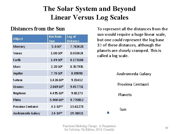
The Solar System and Beyond Linear Versus Log Scales Distances from the Sun Object Km from Sun Log of Distance Mercury 5. 8∙ 107 7. 763428 Venus 1. 08∙ 108 8. 033424 Earth 1. 49∙ 108 8. 173186 Mars 2. 28∙ 108 8. 357935 Jupiter 7. 78∙ 108 8. 89098 Saturn 1. 426∙ 109 9. 15412 Uranus 2. 869∙ 109 9. 457731 Neptune 4. 495∙ 109 9. 65273 Pluto 5. 900∙ 109 9. 770852 Proxima Centauri 4. 1∙ 1013 13. 61278 Andromeda Galaxy 2. 4∙ 1019 19. 38021 To represent all the distances from the sun would require a huge linear scale, but one could represent the log base 10 of these distances, although the planets are closely cramped. This is called a log scale. Functions Modeling Change: A Preparation for Calculus, 5 th Edition, 2014, Connally Andromeda Galaxy Proxima Centauri Planets Sun 36

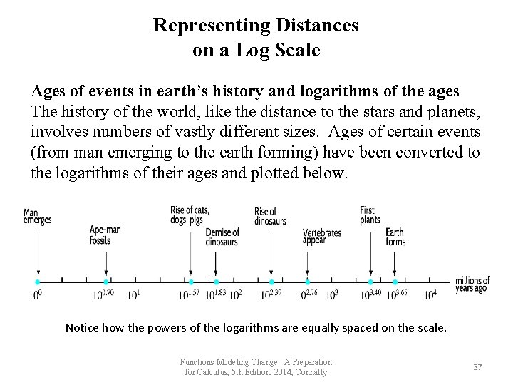
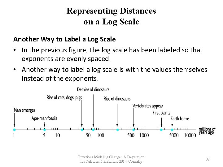
Representing Distances on a Log Scale Ages of events in earth’s history and logarithms of the ages The history of the world, like the distance to the stars and planets, involves numbers of vastly different sizes. Ages of certain events (from man emerging to the earth forming) have been converted to the logarithms of their ages and plotted below. Notice how the powers of the logarithms are equally spaced on the scale. Functions Modeling Change: A Preparation for Calculus, 5 th Edition, 2014, Connally 37

Representing Distances on a Log Scale Another Way to Label a Log Scale • In the previous figure, the log scale has been labeled so that exponents are evenly spaced. • Another way to label a log scale is with the values themselves instead of the exponents. Functions Modeling Change: A Preparation for Calculus, 5 th Edition, 2014, Connally 38

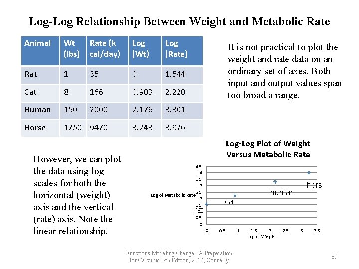
Log-Log Relationship Between Weight and Metabolic Rate Animal Wt (lbs) Rate (k cal/day) Log (Wt) Log (Rate) Rat 1 35 0 1. 544 Cat 8 166 0. 903 2. 220 Human 150 2000 2. 176 3. 301 Horse 1750 9470 3. 243 3. 976 However, we can plot the data using log scales for both the horizontal (weight) axis and the vertical (rate) axis. Note the linear relationship. It is not practical to plot the weight and rate data on an ordinary set of axes. Both input and output values span too broad a range. Log-Log Plot of Weight Versus Metabolic Rate 4. 5 4 3. 5 3 2. 5 Log of Metabolic Rate 2 1. 5 1 0. 5 0 horse human cat rat 0 0. 5 Functions Modeling Change: A Preparation for Calculus, 5 th Edition, 2014, Connally 1 1. 5 2 Log of Weight 2. 5 3 3. 5 39

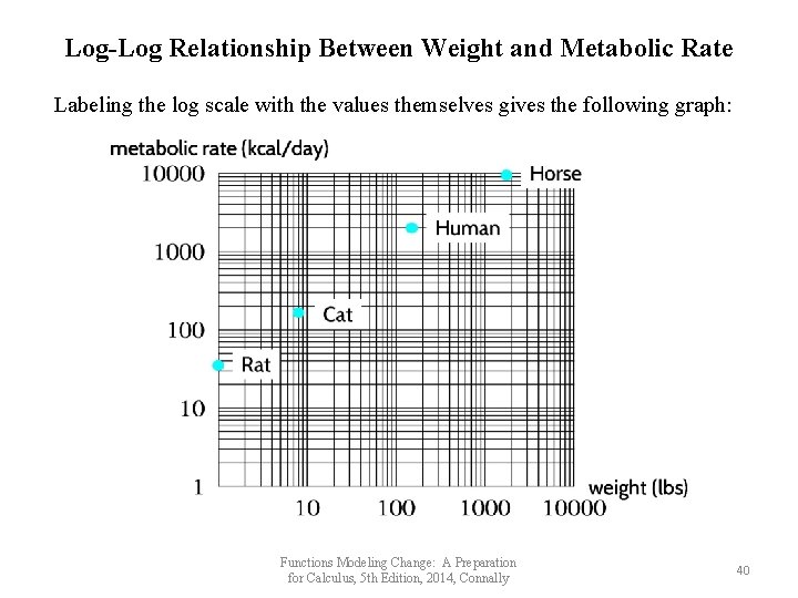
Log-Log Relationship Between Weight and Metabolic Rate Labeling the log scale with the values themselves gives the following graph: Functions Modeling Change: A Preparation for Calculus, 5 th Edition, 2014, Connally 40

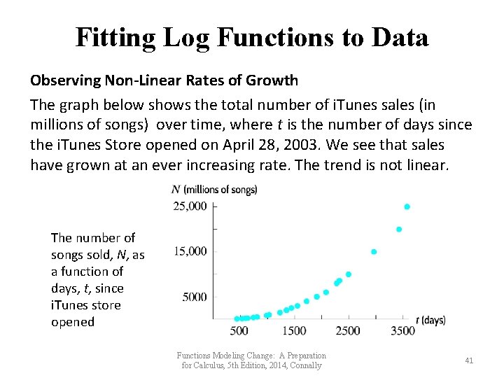
Fitting Log Functions to Data Observing Non-Linear Rates of Growth The graph below shows the total number of i. Tunes sales (in millions of songs) over time, where t is the number of days since the i. Tunes Store opened on April 28, 2003. We see that sales have grown at an ever increasing rate. The trend is not linear. The number of songs sold, N, as a function of days, t, since i. Tunes store opened Functions Modeling Change: A Preparation for Calculus, 5 th Edition, 2014, Connally 41

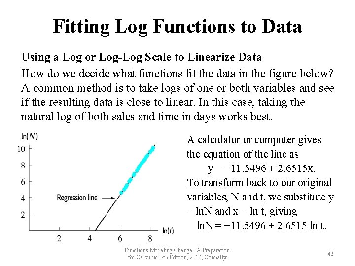
Fitting Log Functions to Data Using a Log or Log-Log Scale to Linearize Data How do we decide what functions fit the data in the figure below? A common method is to take logs of one or both variables and see if the resulting data is close to linear. In this case, taking the natural log of both sales and time in days works best. A calculator or computer gives the equation of the line as y = − 11. 5496 + 2. 6515 x. To transform back to our original variables, N and t, we substitute y = ln. N and x = ln t, giving ln. N = − 11. 5496 + 2. 6515 ln t. Functions Modeling Change: A Preparation for Calculus, 5 th Edition, 2014, Connally 42

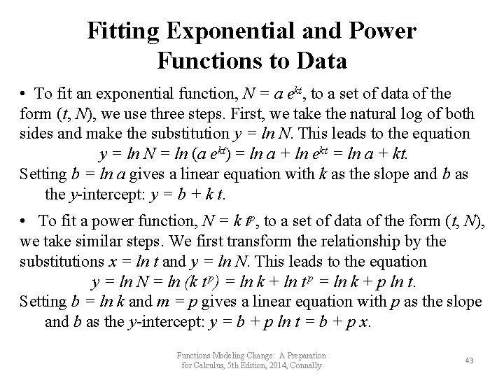
Fitting Exponential and Power Functions to Data • To fit an exponential function, N = a ekt, to a set of data of the form (t, N), we use three steps. First, we take the natural log of both sides and make the substitution y = ln N. This leads to the equation y = ln N = ln (a ekt) = ln a + ln ekt = ln a + kt. Setting b = ln a gives a linear equation with k as the slope and b as the y-intercept: y = b + k t. • To fit a power function, N = k tp, to a set of data of the form (t, N), we take similar steps. We first transform the relationship by the substitutions x = ln t and y = ln N. This leads to the equation y = ln N = ln (k t p) = ln k + ln t p = ln k + p ln t. Setting b = ln k and m = p gives a linear equation with p as the slope and b as the y-intercept: y = b + p ln t = b + p x. Functions Modeling Change: A Preparation for Calculus, 5 th Edition, 2014, Connally 43