Chapter 5 Introduction to Neoclassical Trade Theory Tools

Chapter 5 Introduction to Neoclassical Trade Theory: Tools to Be Employed Mc. Graw-Hill/Irwin Copyright © 2010 by The Mc. Graw-Hill Companies, Inc. All rights reserved.

Learning Objectives § Review the microeconomic principles of consumer and producer behavior. § Explain the concepts and limitations of a community indifference curve. § Examine the underlying basis for a production possibilities frontier with increasing opportunity costs. 5 -2

Consumer Behavior Theory § How do consumers decide how much of each good to consume? 5 -3

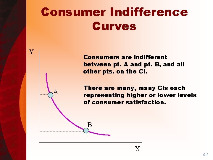
Consumer Indifference Curves Y Consumers are indifferent between pt. A and pt. B, and all other pts. on the CI. A There are many, many CIs each representing higher or lower levels of consumer satisfaction. B X 5 -4

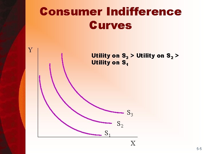
Consumer Indifference Curves Y Utility on S 3 > Utility on S 2 > Utility on S 1 S 3 S 2 S 1 X 5 -5

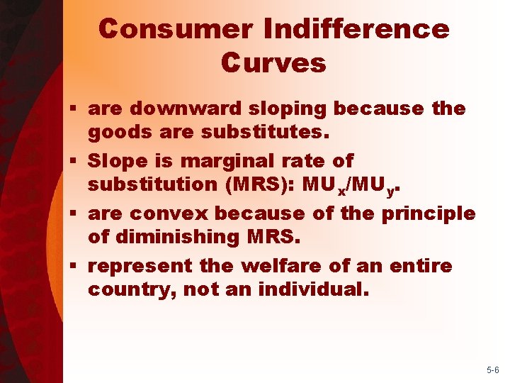
Consumer Indifference Curves § are downward sloping because the goods are substitutes. § Slope is marginal rate of substitution (MRS): MUx/MUy. § are convex because of the principle of diminishing MRS. § represent the welfare of an entire country, not an individual. 5 -6

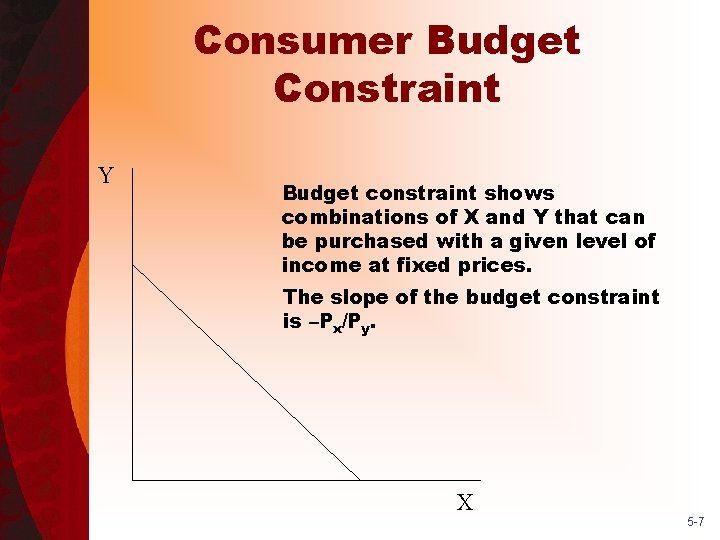
Consumer Budget Constraint Y Budget constraint shows combinations of X and Y that can be purchased with a given level of income at fixed prices. The slope of the budget constraint is –Px/Py. X 5 -7

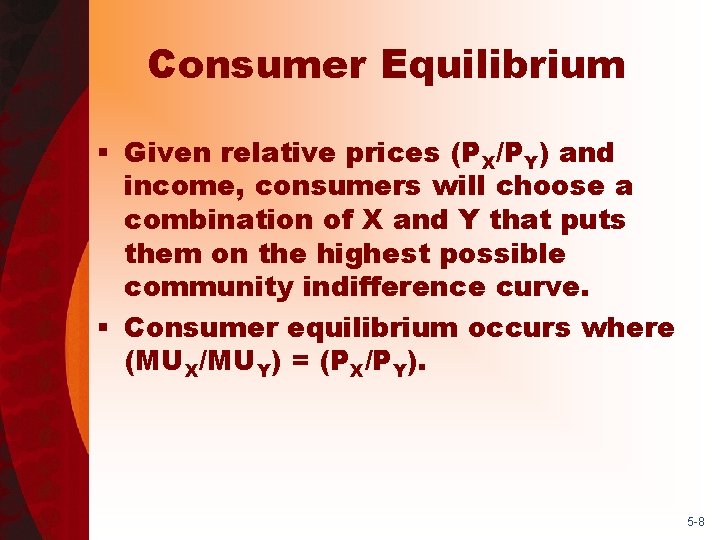
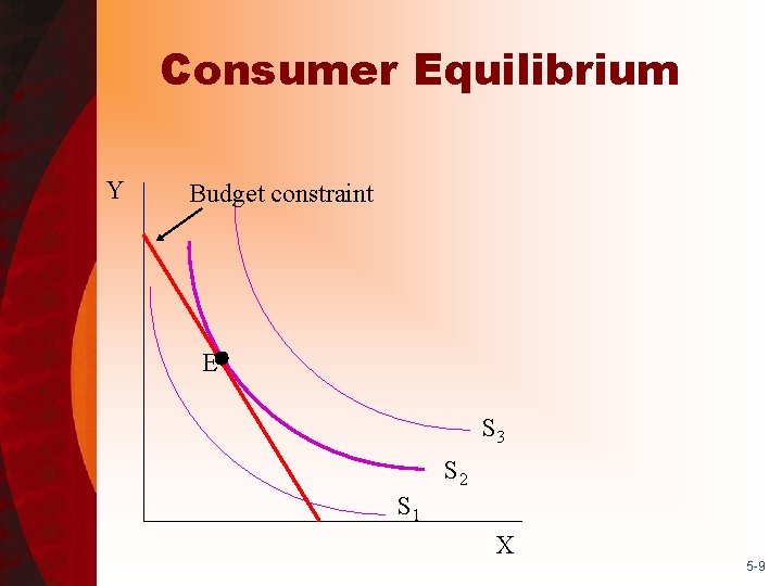
Consumer Equilibrium § Given relative prices (PX/PY) and income, consumers will choose a combination of X and Y that puts them on the highest possible community indifference curve. § Consumer equilibrium occurs where (MUX/MUY) = (PX/PY). 5 -8

Consumer Equilibrium Y Budget constraint E S 3 S 2 S 1 X 5 -9

Production Theory § How do producers choose the mix of inputs to use? § What determines production efficiency within the firm? 5 -10

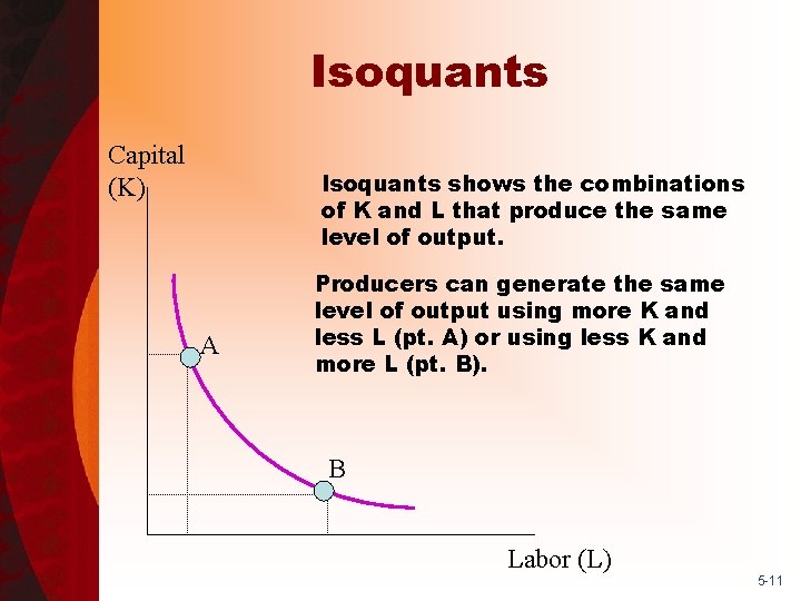
Isoquants Capital (K) Isoquants shows the combinations of K and L that produce the same level of output. A Producers can generate the same level of output using more K and less L (pt. A) or using less K and more L (pt. B). B Labor (L) 5 -11

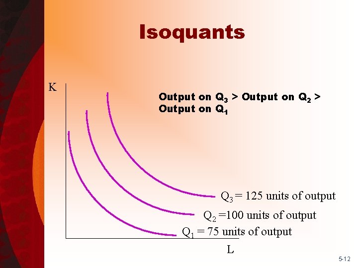
Isoquants K Output on Q 3 > Output on Q 2 > Output on Q 1 Q 3 = 125 units of output Q 2 =100 units of output Q 1 = 75 units of output L 5 -12

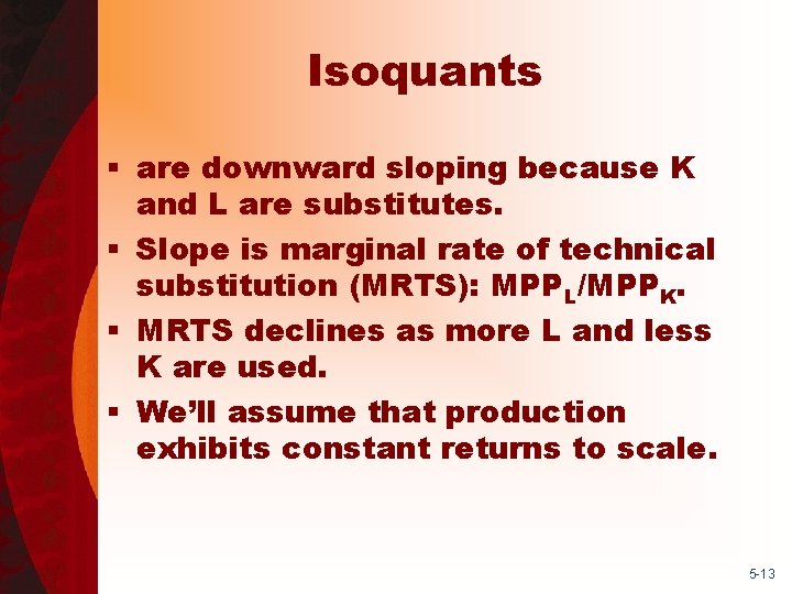
Isoquants § are downward sloping because K and L are substitutes. § Slope is marginal rate of technical substitution (MRTS): MPPL/MPPK. § MRTS declines as more L and less K are used. § We’ll assume that production exhibits constant returns to scale. 5 -13

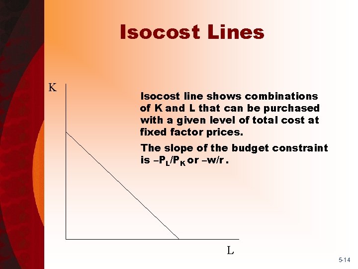
Isocost Lines K Isocost line shows combinations of K and L that can be purchased with a given level of total cost at fixed factor prices. The slope of the budget constraint is –PL/PK or –w/r. L 5 -14

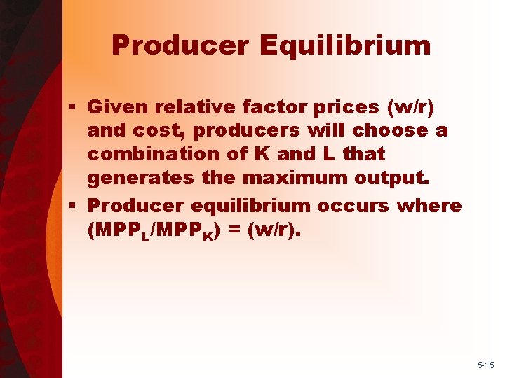
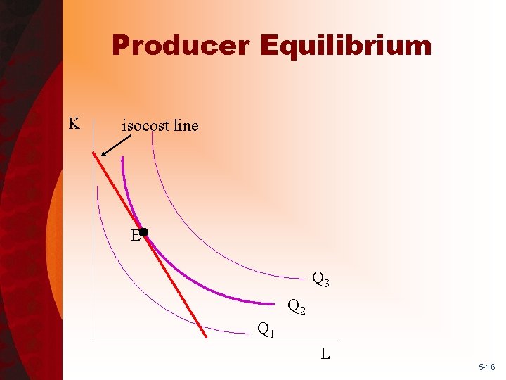
Producer Equilibrium § Given relative factor prices (w/r) and cost, producers will choose a combination of K and L that generates the maximum output. § Producer equilibrium occurs where (MPPL/MPPK) = (w/r). 5 -15

Producer Equilibrium K isocost line E Q 3 Q 2 Q 1 L 5 -16

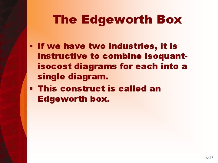
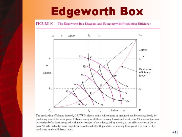
The Edgeworth Box § If we have two industries, it is instructive to combine isoquantisocost diagrams for each into a single diagram. § This construct is called an Edgeworth box. 5 -17

Edgeworth Box 5 -18

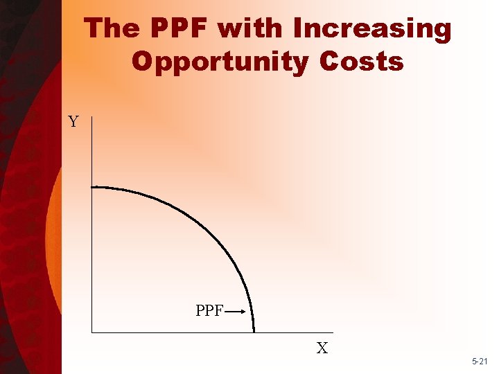
Production Possibilities Frontier § Most PPFs are bowed out, not straight lines. § This is because resources are not equally suited to all kinds of production. 5 -19

Production Possibilities Frontier § Slope of a tangent line at any point along the PPF is: • the marginal rate of transformation, or • the opportunity cost of the horizontal axis good, or • MCX/MCY. 5 -20

The PPF with Increasing Opportunity Costs Y PPF X 5 -21