Chapter 5 Divide and Conquer Slides by Kevin
Chapter 5 Divide and Conquer Slides by Kevin Wayne. Copyright © 2005 Pearson-Addison Wesley. All rights reserved. 1
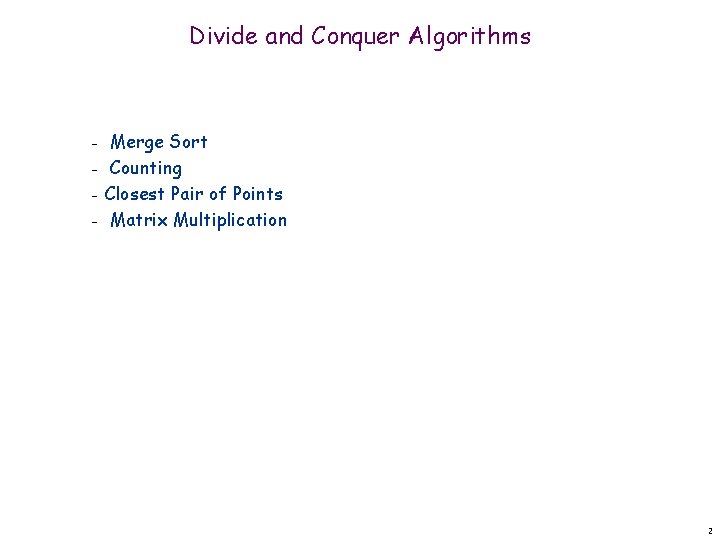
Divide and Conquer Algorithms Merge Sort - Counting - Closest Pair of Points - Matrix Multiplication - 2
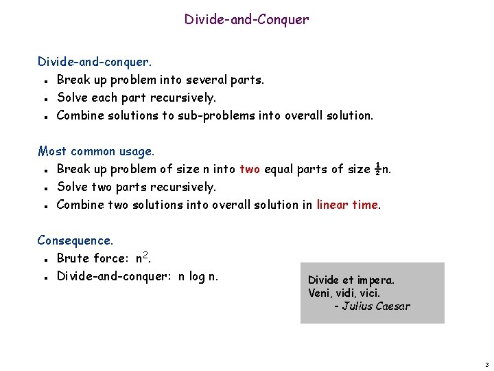
Divide-and-Conquer Divide-and-conquer. Break up problem into several parts. Solve each part recursively. Combine solutions to sub-problems into overall solution. n n n Most common usage. Break up problem of size n into two equal parts of size ½n. Solve two parts recursively. Combine two solutions into overall solution in linear time. n n n Consequence. Brute force: n 2. Divide-and-conquer: n log n. n n Divide et impera. Veni, vidi, vici. - Julius Caesar 3
5. 1 Mergesort
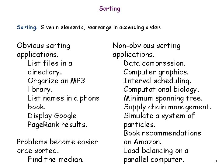
Sorting. Given n elements, rearrange in ascending order. Obvious sorting applications. List files in a directory. Organize an MP 3 library. List names in a phone book. Display Google Page. Rank results. Problems become easier once sorted. Find the median. Non-obvious sorting applications. Data compression. Computer graphics. Interval scheduling. Computational biology. Minimum spanning tree. Supply chain management. Simulate a system of particles. Book recommendations on Amazon. Load balancing on a parallel computer. 5
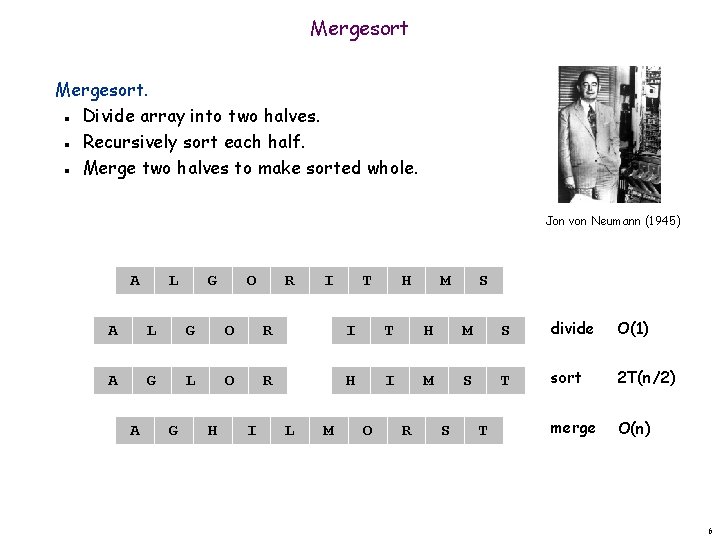
Mergesort. Divide array into two halves. Recursively sort each half. Merge two halves to make sorted whole. n n n Jon von Neumann (1945) A L G O R I T H M S divide O(1) A G L O R H I M S T sort 2 T(n/2) merge O(n) A G H I L M O R S T 6
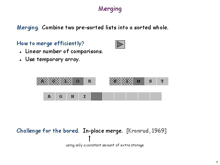
Merging. Combine two pre-sorted lists into a sorted whole. How to merge efficiently? Linear number of comparisons. Use temporary array. n n A G A L G O H R H I M S T I Challenge for the bored. In-place merge. [Kronrud, 1969] using only a constant amount of extra storage 7
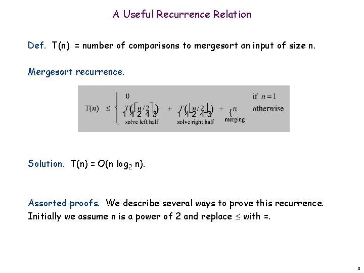
A Useful Recurrence Relation Def. T(n) = number of comparisons to mergesort an input of size n. Mergesort recurrence. Solution. T(n) = O(n log 2 n). Assorted proofs. We describe several ways to prove this recurrence. Initially we assume n is a power of 2 and replace with =. 8
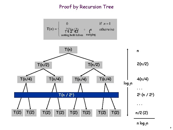
Proof by Recursion Tree T(n) n T(n/4) 2(n/2) T(n/2) T(n/4) log 2 n 4(n/4). . . 2 k (n / 2 k) T(n / 2 k) . . . T(2) T(2) n/2 (2) n log 2 n 9
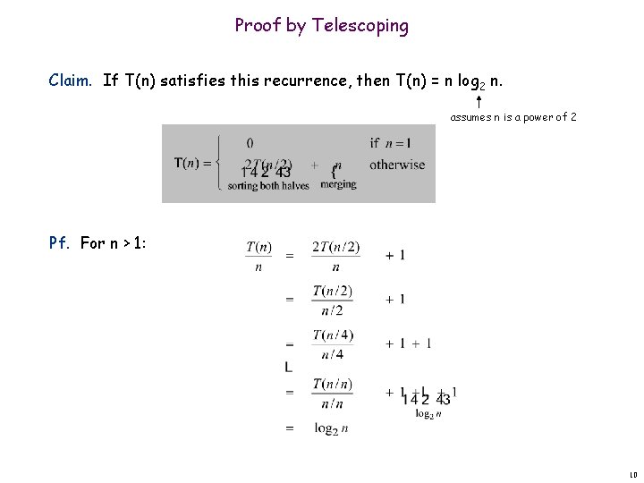
Proof by Telescoping Claim. If T(n) satisfies this recurrence, then T(n) = n log 2 n. assumes n is a power of 2 Pf. For n > 1: 10
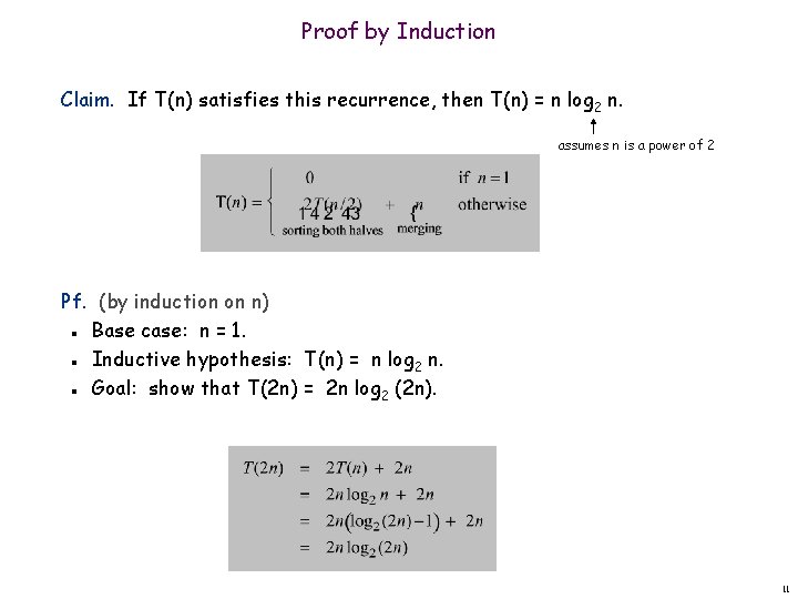
Proof by Induction Claim. If T(n) satisfies this recurrence, then T(n) = n log 2 n. assumes n is a power of 2 Pf. (by induction on n) Base case: n = 1. Inductive hypothesis: T(n) = n log 2 n. Goal: show that T(2 n) = 2 n log 2 (2 n). n n n 11
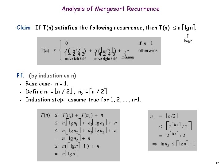
Analysis of Mergesort Recurrence Claim. If T(n) satisfies the following recurrence, then T(n) n lg n. log 2 n Pf. (by induction on n) Base case: n = 1. Define n 1 = n / 2 , n 2 = n / 2. Induction step: assume true for 1, 2, . . . , n– 1. n n n 12
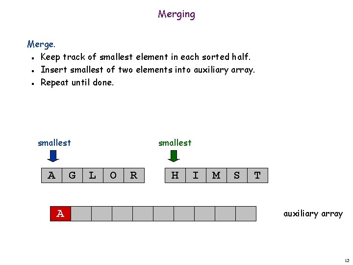
Merging Merge. Keep track of smallest element in each sorted half. Insert smallest of two elements into auxiliary array. Repeat until done. n n n smallest A G A smallest L O R H I M S T auxiliary array 13
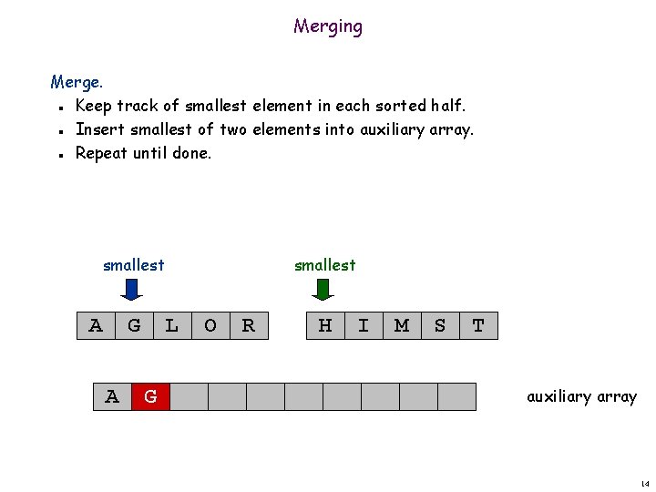
Merging Merge. Keep track of smallest element in each sorted half. Insert smallest of two elements into auxiliary array. Repeat until done. n n n smallest A G A smallest L G O R H I M S T auxiliary array 14
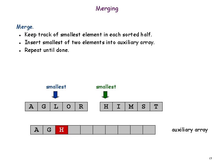
Merging Merge. Keep track of smallest element in each sorted half. Insert smallest of two elements into auxiliary array. Repeat until done. n n n smallest A G A L G smallest O H R H I M S T auxiliary array 15
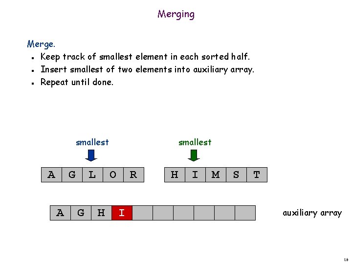
Merging Merge. Keep track of smallest element in each sorted half. Insert smallest of two elements into auxiliary array. Repeat until done. n n n smallest A G A L G smallest O H R I H I M S T auxiliary array 16
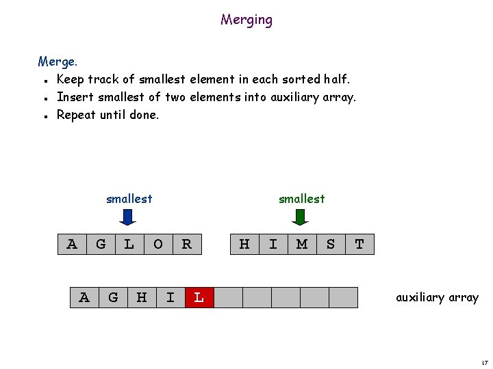
Merging Merge. Keep track of smallest element in each sorted half. Insert smallest of two elements into auxiliary array. Repeat until done. n n n smallest A G A L G smallest O H R I H L I M S T auxiliary array 17
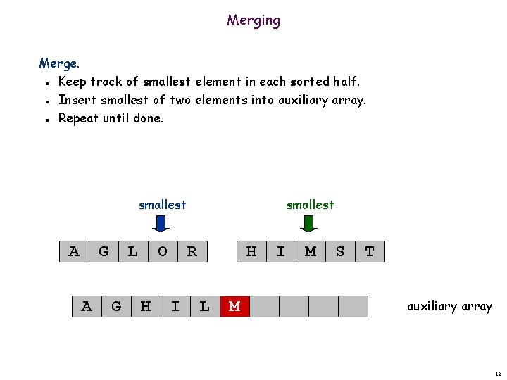
Merging Merge. Keep track of smallest element in each sorted half. Insert smallest of two elements into auxiliary array. Repeat until done. n n n smallest A G A L G O H smallest R I H L M I M S T auxiliary array 18
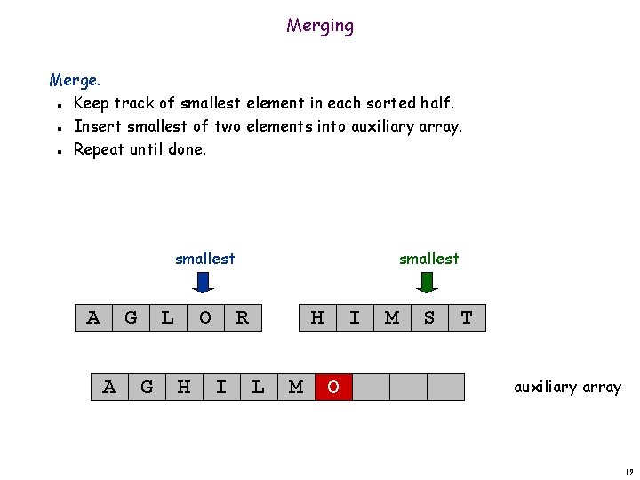
Merging Merge. Keep track of smallest element in each sorted half. Insert smallest of two elements into auxiliary array. Repeat until done. n n n smallest A G A L G O H smallest R I H L M I O M S T auxiliary array 19

Merging Merge. Keep track of smallest element in each sorted half. Insert smallest of two elements into auxiliary array. Repeat until done. n n n smallest A G A L G O H smallest R I H L M I O M R S T auxiliary array 20
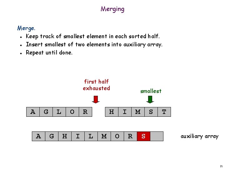
Merging Merge. Keep track of smallest element in each sorted half. Insert smallest of two elements into auxiliary array. Repeat until done. n n n first half exhausted A G A L G O H R I smallest H L M I O M R S S T auxiliary array 21
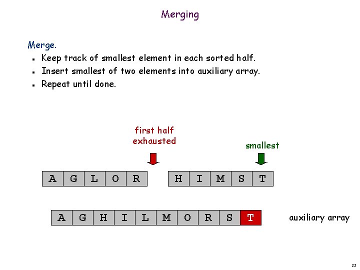
Merging Merge. Keep track of smallest element in each sorted half. Insert smallest of two elements into auxiliary array. Repeat until done. n n n first half exhausted A G A L G O H R I smallest H L M I O M R S S T T auxiliary array 22
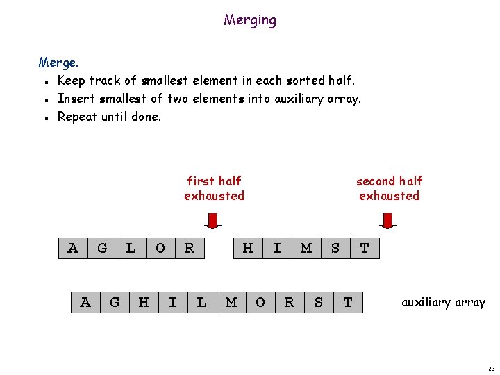
Merging Merge. Keep track of smallest element in each sorted half. Insert smallest of two elements into auxiliary array. Repeat until done. n n n first half exhausted A G A L G O H R I second half exhausted H L M I O M R S S T T auxiliary array 23
5. 3 Counting Inversions
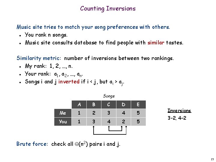
Counting Inversions Music site tries to match your song preferences with others. You rank n songs. Music site consults database to find people with similar tastes. n n Similarity metric: number of inversions between two rankings. My rank: 1, 2, …, n. Your rank: a 1, a 2, …, an. Songs i and j inverted if i < j, but ai > aj. n n n Songs A B C D E Me 1 2 3 4 5 You 1 3 4 2 5 Inversions 3 -2, 4 -2 Brute force: check all (n 2) pairs i and j. 25
Applications. Voting theory. Collaborative filtering. Measuring the "sortedness" of an array. Sensitivity analysis of Google's ranking function. Rank aggregation for meta-searching on the Web. Nonparametric statistics (e. g. , Kendall's Tau distance). n n n 26
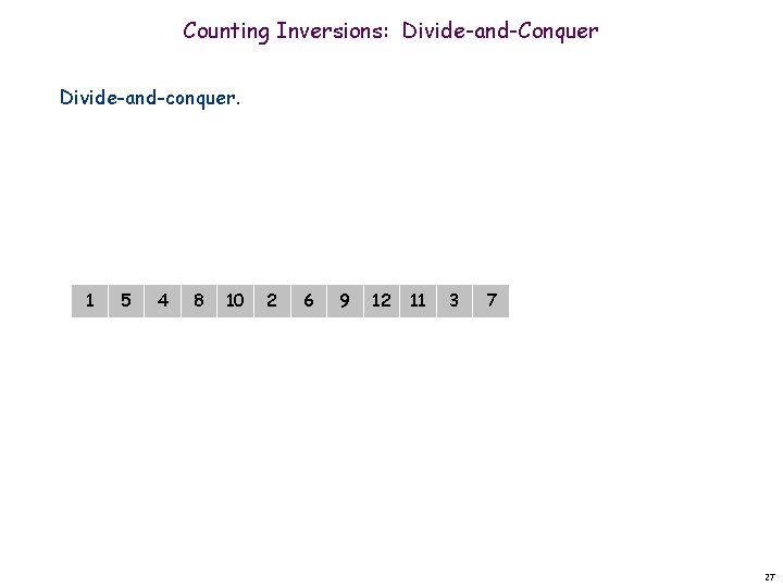
Counting Inversions: Divide-and-Conquer Divide-and-conquer. 1 5 4 8 10 2 6 9 12 11 3 7 27
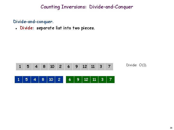
Counting Inversions: Divide-and-Conquer Divide-and-conquer. Divide: separate list into two pieces. n 1 1 5 5 4 4 8 8 10 10 2 2 6 6 9 9 12 12 11 11 3 3 7 Divide: O(1). 7 28
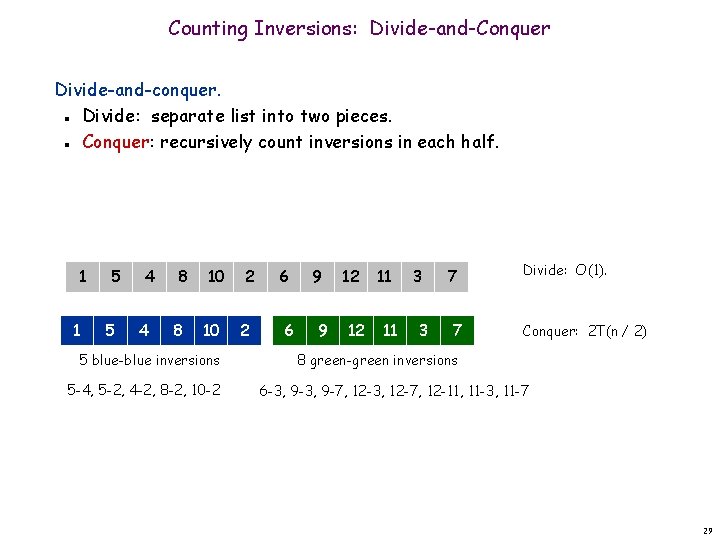
Counting Inversions: Divide-and-Conquer Divide-and-conquer. Divide: separate list into two pieces. Conquer: recursively count inversions in each half. n n 1 1 5 5 4 4 8 8 10 10 5 blue-blue inversions 5 -4, 5 -2, 4 -2, 8 -2, 10 -2 2 2 6 6 9 9 12 12 11 11 3 3 7 7 Divide: O(1). Conquer: 2 T(n / 2) 8 green-green inversions 6 -3, 9 -7, 12 -3, 12 -7, 12 -11, 11 -3, 11 -7 29
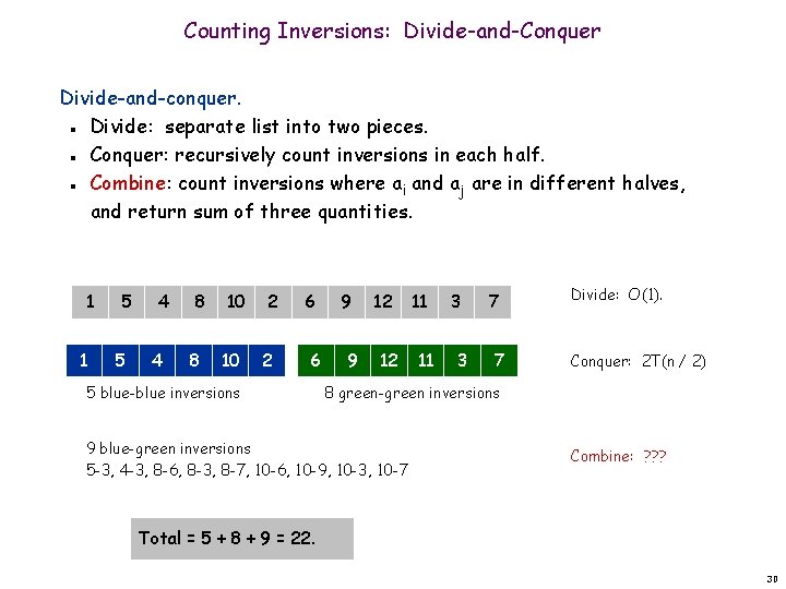
Counting Inversions: Divide-and-Conquer Divide-and-conquer. Divide: separate list into two pieces. Conquer: recursively count inversions in each half. Combine: count inversions where ai and aj are in different halves, and return sum of three quantities. n n n 1 1 5 5 4 4 8 8 10 10 2 2 6 6 5 blue-blue inversions 9 9 12 12 11 11 3 3 7 7 Divide: O(1). Conquer: 2 T(n / 2) 8 green-green inversions 9 blue-green inversions 5 -3, 4 -3, 8 -6, 8 -3, 8 -7, 10 -6, 10 -9, 10 -3, 10 -7 Combine: ? ? ? Total = 5 + 8 + 9 = 22. 30
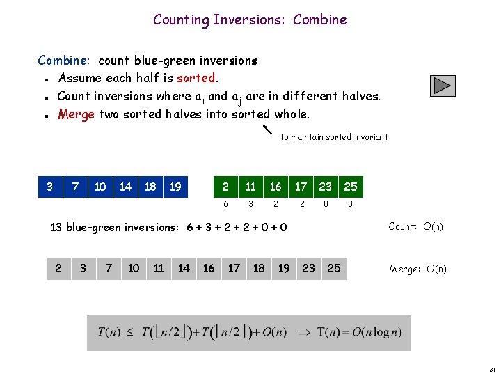
Counting Inversions: Combine: count blue-green inversions Assume each half is sorted. Count inversions where ai and aj are in different halves. Merge two sorted halves into sorted whole. n n n to maintain sorted invariant 3 7 10 14 18 19 2 11 16 17 23 25 6 3 2 2 0 0 13 blue-green inversions: 6 + 3 + 2 + 0 2 3 7 10 11 14 16 17 18 19 Count: O(n) 23 25 Merge: O(n) 31
![Counting Inversions: Implementation Pre-condition. [Merge-and-Count] A and B are sorted. Post-condition. [Sort-and-Count] L is Counting Inversions: Implementation Pre-condition. [Merge-and-Count] A and B are sorted. Post-condition. [Sort-and-Count] L is](http://slidetodoc.com/presentation_image_h2/fd20ffb51f9745660af0278313113a89/image-32.jpg)
Counting Inversions: Implementation Pre-condition. [Merge-and-Count] A and B are sorted. Post-condition. [Sort-and-Count] L is sorted. Sort-and-Count(L) { if list L has one element return 0 and the list L Divide the list into two halves A and B (r. A, A) Sort-and-Count(A) (r. B, B) Sort-and-Count(B) (r. B, L) Merge-and-Count(A, B) } return r = r. A + r. B + r and the sorted list L 32
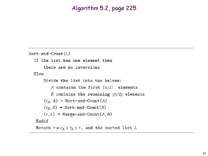
Algorithm 5. 2, page 225 33
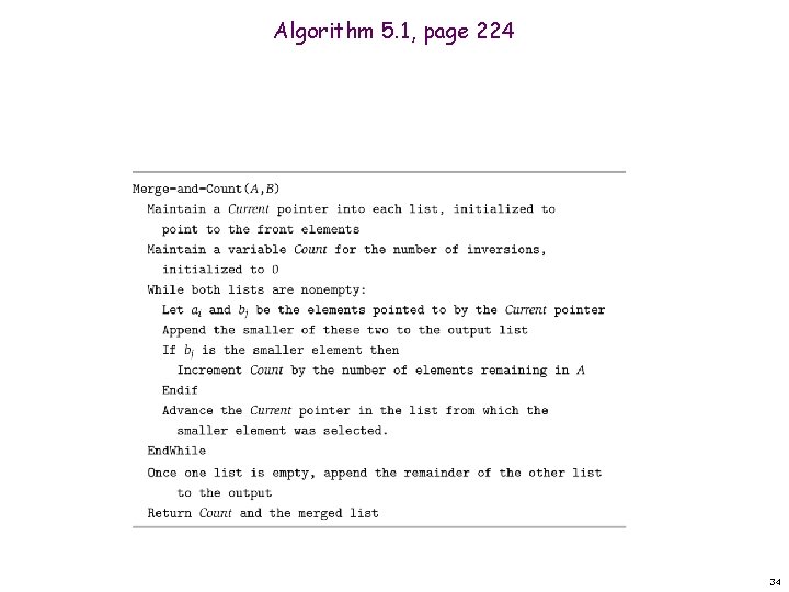
Algorithm 5. 1, page 224 34

Merge and Count Merge and count step. Given two sorted halves, count number of inversions where ai and aj are in different halves. Combine two sorted halves into sorted whole. n n i=6 3 7 10 14 18 19 2 11 16 17 23 25 two sorted halves auxiliary array Total: 35
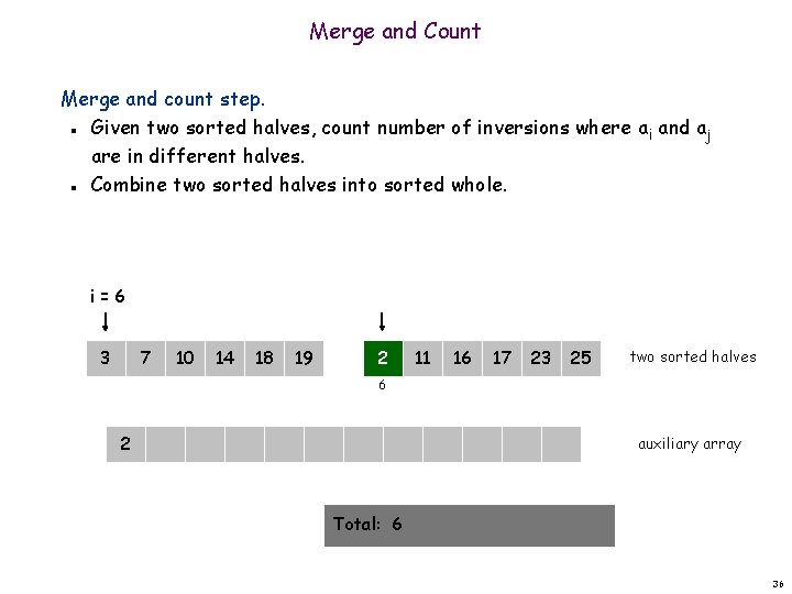
Merge and Count Merge and count step. Given two sorted halves, count number of inversions where ai and aj are in different halves. Combine two sorted halves into sorted whole. n n i=6 3 7 10 14 18 19 2 11 16 17 23 25 two sorted halves 6 2 auxiliary array Total: 6 36

Merge and Count Merge and count step. Given two sorted halves, count number of inversions where ai and aj are in different halves. Combine two sorted halves into sorted whole. n n i=6 3 7 10 14 18 19 2 11 16 17 23 25 two sorted halves 6 2 auxiliary array Total: 6 37
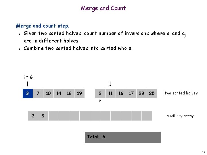
Merge and Count Merge and count step. Given two sorted halves, count number of inversions where ai and aj are in different halves. Combine two sorted halves into sorted whole. n n i=6 3 7 10 14 18 19 2 11 16 17 23 25 two sorted halves 6 2 3 auxiliary array Total: 6 38
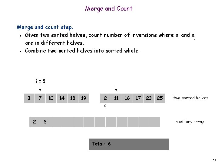
Merge and Count Merge and count step. Given two sorted halves, count number of inversions where ai and aj are in different halves. Combine two sorted halves into sorted whole. n n i=5 3 7 10 14 18 19 2 11 16 17 23 25 two sorted halves 6 2 3 auxiliary array Total: 6 39
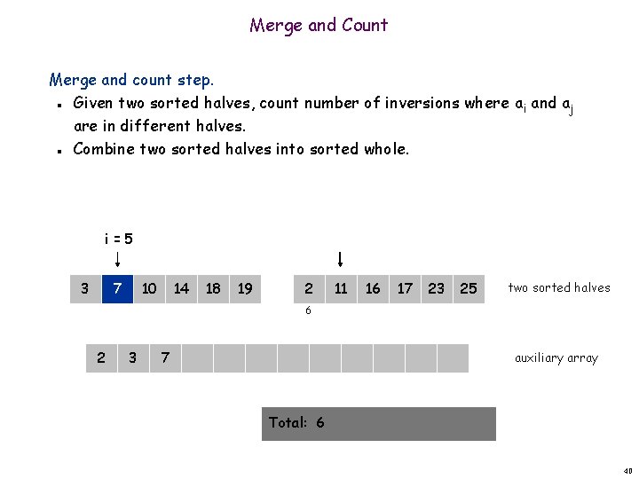
Merge and Count Merge and count step. Given two sorted halves, count number of inversions where ai and aj are in different halves. Combine two sorted halves into sorted whole. n n i=5 3 7 10 14 18 19 2 11 16 17 23 25 two sorted halves 6 2 3 7 auxiliary array Total: 6 40
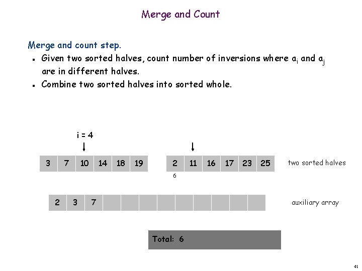
Merge and Count Merge and count step. Given two sorted halves, count number of inversions where ai and aj are in different halves. Combine two sorted halves into sorted whole. n n i=4 3 7 10 14 18 19 2 11 16 17 23 25 two sorted halves 6 2 3 7 auxiliary array Total: 6 41
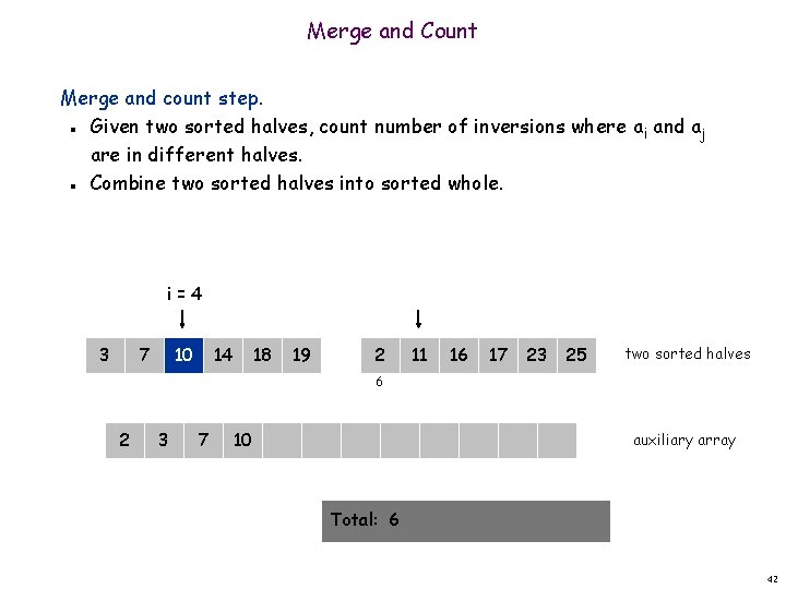
Merge and Count Merge and count step. Given two sorted halves, count number of inversions where ai and aj are in different halves. Combine two sorted halves into sorted whole. n n i=4 3 7 10 14 18 19 2 11 16 17 23 25 two sorted halves 6 2 3 7 10 auxiliary array Total: 6 42

Merge and Count Merge and count step. Given two sorted halves, count number of inversions where ai and aj are in different halves. Combine two sorted halves into sorted whole. n n i=3 3 7 10 14 18 19 2 11 16 17 23 25 two sorted halves 6 2 3 7 10 auxiliary array Total: 6 43
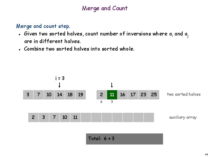
Merge and Count Merge and count step. Given two sorted halves, count number of inversions where ai and aj are in different halves. Combine two sorted halves into sorted whole. n n i=3 3 7 2 10 3 14 7 18 10 19 2 11 6 3 11 16 17 23 25 two sorted halves auxiliary array Total: 6 + 3 44

Merge and Count Merge and count step. Given two sorted halves, count number of inversions where ai and aj are in different halves. Combine two sorted halves into sorted whole. n n i=3 3 7 2 10 3 14 7 18 10 19 2 11 6 3 11 16 17 23 25 two sorted halves auxiliary array Total: 6 + 3 45
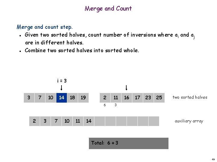
Merge and Count Merge and count step. Given two sorted halves, count number of inversions where ai and aj are in different halves. Combine two sorted halves into sorted whole. n n i=3 3 7 2 10 3 14 7 18 10 19 11 2 11 6 3 14 16 17 23 25 two sorted halves auxiliary array Total: 6 + 3 46

Merge and Count Merge and count step. Given two sorted halves, count number of inversions where ai and aj are in different halves. Combine two sorted halves into sorted whole. n n i=2 3 7 2 10 3 14 7 18 10 19 11 2 11 6 3 14 16 17 23 25 two sorted halves auxiliary array Total: 6 + 3 47
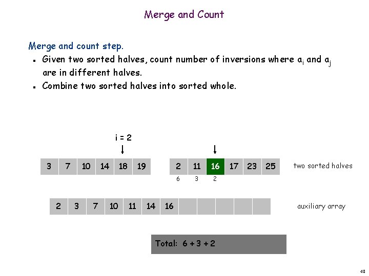
Merge and Count Merge and count step. Given two sorted halves, count number of inversions where ai and aj are in different halves. Combine two sorted halves into sorted whole. n n i=2 3 7 2 10 3 14 7 18 10 19 11 14 2 11 16 6 3 2 16 17 23 25 two sorted halves auxiliary array Total: 6 + 3 + 2 48
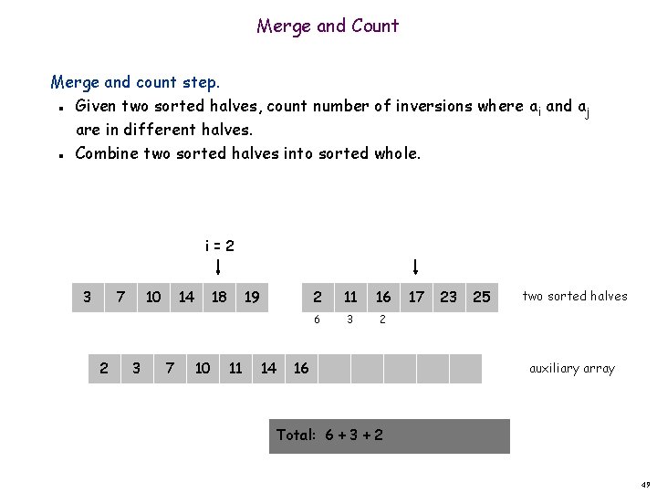
Merge and Count Merge and count step. Given two sorted halves, count number of inversions where ai and aj are in different halves. Combine two sorted halves into sorted whole. n n i=2 3 7 2 10 3 14 7 18 10 19 11 14 2 11 16 6 3 2 16 17 23 25 two sorted halves auxiliary array Total: 6 + 3 + 2 49
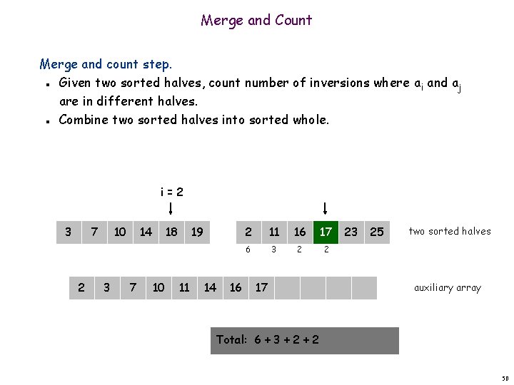
Merge and Count Merge and count step. Given two sorted halves, count number of inversions where ai and aj are in different halves. Combine two sorted halves into sorted whole. n n i=2 3 7 2 10 3 14 7 18 10 19 11 14 16 2 11 16 17 6 3 2 2 17 23 25 two sorted halves auxiliary array Total: 6 + 3 + 2 50

Merge and Count Merge and count step. Given two sorted halves, count number of inversions where ai and aj are in different halves. Combine two sorted halves into sorted whole. n n i=2 3 7 2 10 3 14 7 18 10 19 11 14 16 2 11 16 17 6 3 2 2 17 23 25 two sorted halves auxiliary array Total: 6 + 3 + 2 51
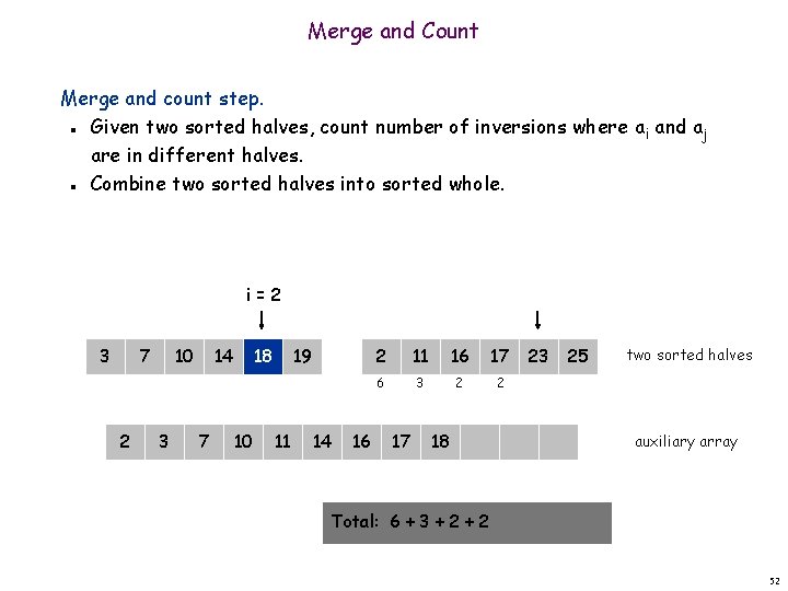
Merge and Count Merge and count step. Given two sorted halves, count number of inversions where ai and aj are in different halves. Combine two sorted halves into sorted whole. n n i=2 3 7 2 10 3 14 7 18 10 19 11 14 16 2 11 16 17 6 3 2 2 17 18 23 25 two sorted halves auxiliary array Total: 6 + 3 + 2 52
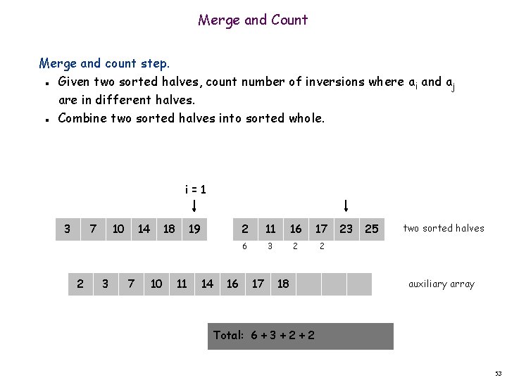
Merge and Count Merge and count step. Given two sorted halves, count number of inversions where ai and aj are in different halves. Combine two sorted halves into sorted whole. n n i=1 3 7 2 10 3 14 7 18 10 19 11 14 16 2 11 16 17 6 3 2 2 17 18 23 25 two sorted halves auxiliary array Total: 6 + 3 + 2 53
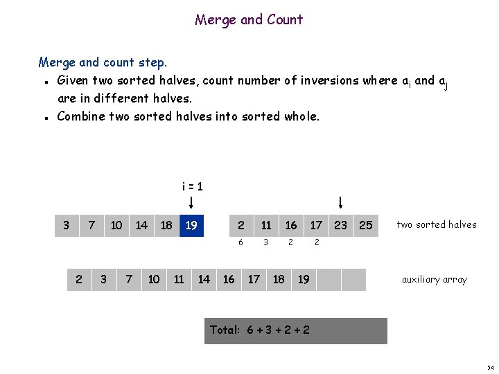
Merge and Count Merge and count step. Given two sorted halves, count number of inversions where ai and aj are in different halves. Combine two sorted halves into sorted whole. n n i=1 3 7 2 10 3 14 7 18 10 19 11 14 16 2 11 16 17 6 3 2 2 17 18 19 23 25 two sorted halves auxiliary array Total: 6 + 3 + 2 54
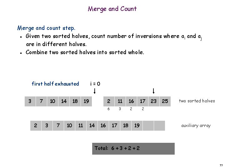
Merge and Count Merge and count step. Given two sorted halves, count number of inversions where ai and aj are in different halves. Combine two sorted halves into sorted whole. n n first half exhausted 3 7 2 10 3 14 7 18 10 i=0 19 11 14 16 2 11 16 17 6 3 2 2 17 18 19 23 25 two sorted halves auxiliary array Total: 6 + 3 + 2 55
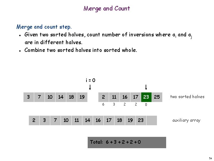
Merge and Count Merge and count step. Given two sorted halves, count number of inversions where ai and aj are in different halves. Combine two sorted halves into sorted whole. n n i=0 3 7 2 10 3 14 7 18 10 19 11 14 16 2 11 16 17 23 6 3 2 2 0 17 18 19 23 25 two sorted halves auxiliary array Total: 6 + 3 + 2 + 0 56

Merge and Count Merge and count step. Given two sorted halves, count number of inversions where ai and aj are in different halves. Combine two sorted halves into sorted whole. n n i=0 3 7 2 10 3 14 7 18 10 19 11 14 16 2 11 16 17 23 6 3 2 2 0 17 18 19 23 25 two sorted halves auxiliary array Total: 6 + 3 + 2 + 0 57
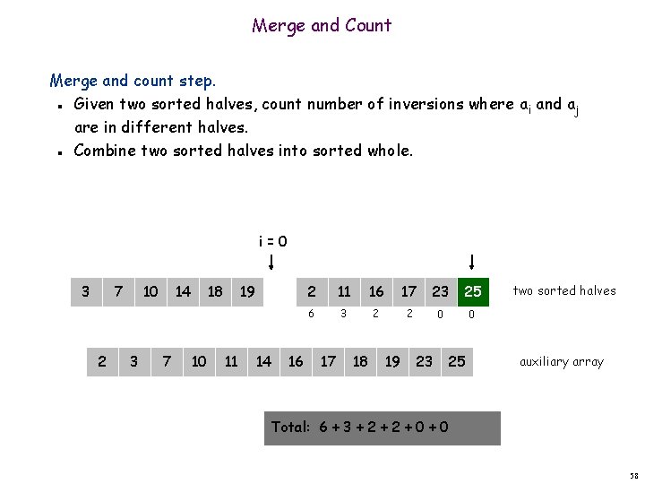
Merge and Count Merge and count step. Given two sorted halves, count number of inversions where ai and aj are in different halves. Combine two sorted halves into sorted whole. n n i=0 3 7 2 10 3 14 7 18 10 19 11 14 16 2 11 16 17 23 25 6 3 2 2 0 0 17 18 19 23 25 two sorted halves auxiliary array Total: 6 + 3 + 2 + 0 58

Merge and Count Merge and count step. Given two sorted halves, count number of inversions where ai and aj are in different halves. Combine two sorted halves into sorted whole. n n i=0 3 7 2 10 3 14 7 18 10 19 11 14 16 2 11 16 17 23 25 6 3 2 2 0 0 17 18 19 23 25 two sorted halves auxiliary array Total: 6 + 3 + 2 + 0 = 13 59
Closest Pair of Points Closest pair. Given n points in the plane, find a pair with smallest Euclidean distance between them. Fundamental geometric primitive. Graphics, computer vision, geographic information systems, molecular modeling, air traffic control. Special case of nearest neighbor, Euclidean MST, Voronoi. n n fast closest pair inspired fast algorithms for these problems Brute force. Check all pairs of points p and q with (n 2) comparisons. 1 -D version. O(n log n) easy if points are on a line. Assumption. No two points have same x coordinate. to make presentation cleaner 60
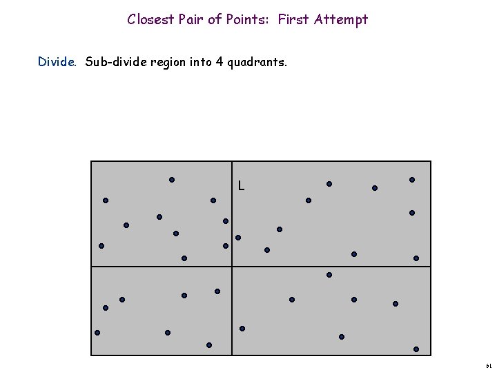
Closest Pair of Points: First Attempt Divide. Sub-divide region into 4 quadrants. L 61
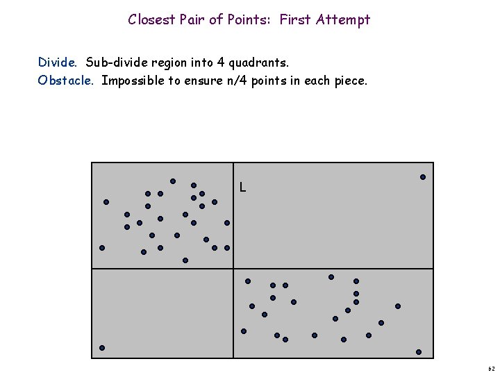
Closest Pair of Points: First Attempt Divide. Sub-divide region into 4 quadrants. Obstacle. Impossible to ensure n/4 points in each piece. L 62
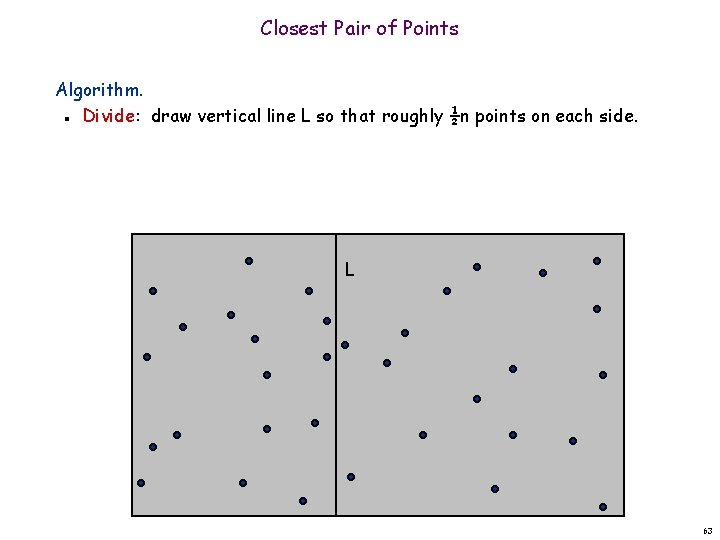
Closest Pair of Points Algorithm. Divide: draw vertical line L so that roughly ½n points on each side. n L 63
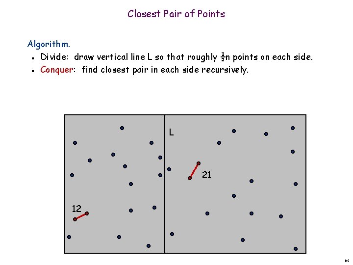
Closest Pair of Points Algorithm. Divide: draw vertical line L so that roughly ½n points on each side. Conquer: find closest pair in each side recursively. n n L 21 12 64
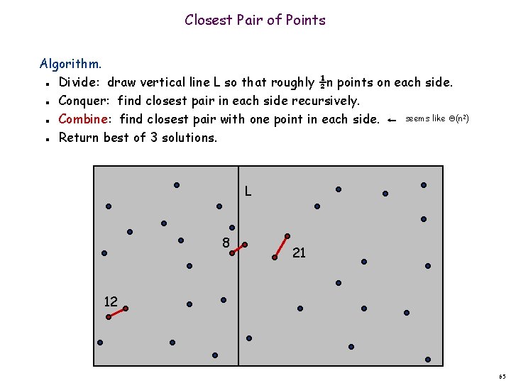
Closest Pair of Points Algorithm. Divide: draw vertical line L so that roughly ½n points on each side. Conquer: find closest pair in each side recursively. seems like (n 2) Combine: find closest pair with one point in each side. Return best of 3 solutions. n n L 8 21 12 65
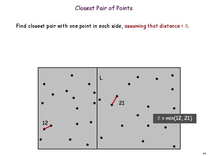
Closest Pair of Points Find closest pair with one point in each side, assuming that distance < . L 21 12 = min(12, 21) 66
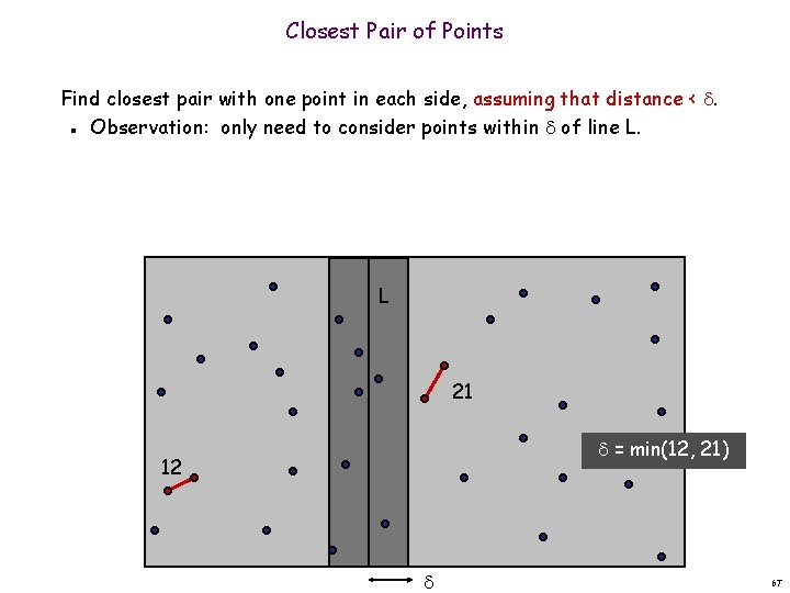
Closest Pair of Points Find closest pair with one point in each side, assuming that distance < . Observation: only need to consider points within of line L. n L 21 = min(12, 21) 12 67
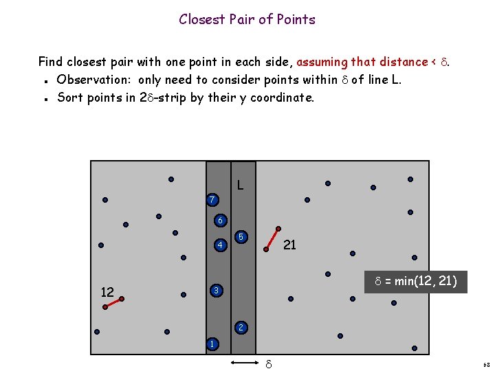
Closest Pair of Points Find closest pair with one point in each side, assuming that distance < . Observation: only need to consider points within of line L. Sort points in 2 -strip by their y coordinate. n n L 7 6 4 12 5 21 = min(12, 21) 3 2 1 68
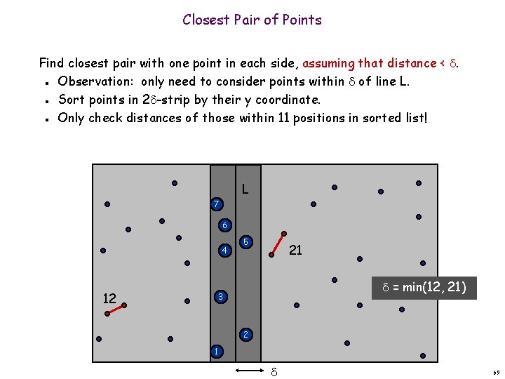
Closest Pair of Points Find closest pair with one point in each side, assuming that distance < . Observation: only need to consider points within of line L. Sort points in 2 -strip by their y coordinate. Only check distances of those within 11 positions in sorted list! n n n L 7 6 4 12 5 21 = min(12, 21) 3 2 1 69
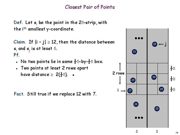
Closest Pair of Points Def. Let si be the point in the 2 -strip, with the ith smallest y-coordinate. Claim. If |i – j| 12, then the distance between si and sj is at least . Pf. No two points lie in same ½ -by-½ box. Two points at least 2 rows apart 2 rows have distance 2(½ ). ▪ j 39 31 n ½ n Fact. Still true if we replace 12 with 7. i ½ 30 29 28 27 ½ 26 25 70
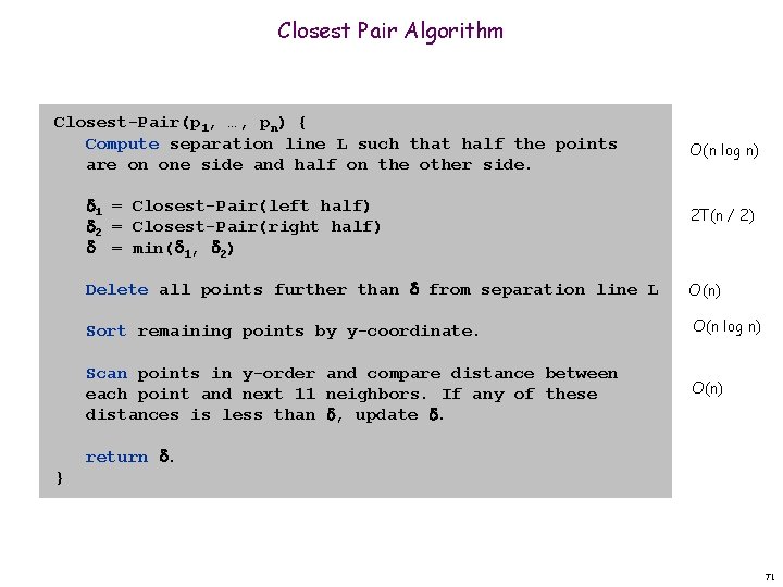
Closest Pair Algorithm Closest-Pair(p 1, …, pn) { Compute separation line L such that half the points are on one side and half on the other side. 1 = Closest-Pair(left half) 2 = Closest-Pair(right half) = min( 1, 2) O(n log n) 2 T(n / 2) Delete all points further than from separation line L O(n) Sort remaining points by y-coordinate. O(n log n) Scan points in y-order and compare distance between each point and next 11 neighbors. If any of these distances is less than , update . O(n) return . } 71
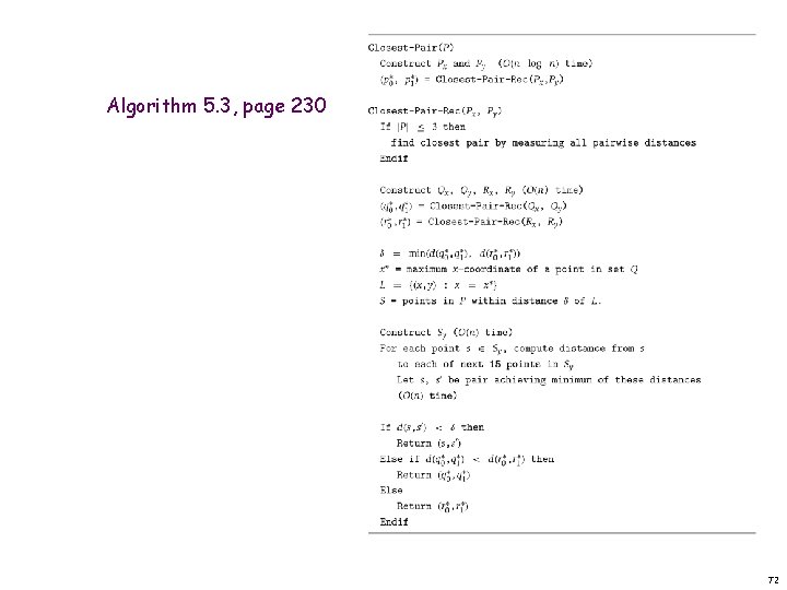
Algorithm 5. 3, page 230 72

Closest Pair of Points: Analysis Running time. Q. Can we achieve O(n log n)? A. Yes. Don't sort points in strip from scratch each time. Each recursive returns two lists: all points sorted by y coordinate, and all points sorted by x coordinate. Sort by merging two pre-sorted lists. n n 73
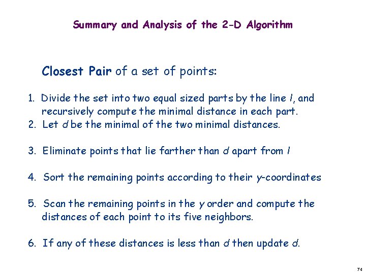
Summary and Analysis of the 2 -D Algorithm Closest Pair of a set of points: 1. Divide the set into two equal sized parts by the line l, and recursively compute the minimal distance in each part. 2. Let d be the minimal of the two minimal distances. 3. Eliminate points that lie farther than d apart from l 4. Sort the remaining points according to their y-coordinates 5. Scan the remaining points in the y order and compute the distances of each point to its five neighbors. 6. If any of these distances is less than d then update d. 74
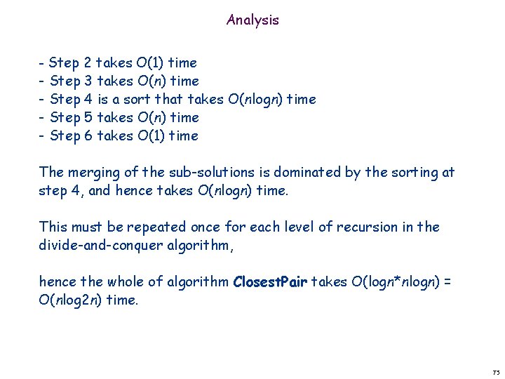
Analysis - Step 2 takes O(1) time - Step 3 takes O(n) time - Step 4 is a sort that takes O(nlogn) time - Step 5 takes O(n) time - Step 6 takes O(1) time The merging of the sub-solutions is dominated by the sorting at step 4, and hence takes O(nlogn) time. This must be repeated once for each level of recursion in the divide-and-conquer algorithm, hence the whole of algorithm Closest. Pair takes O(logn*nlogn) = O(nlog 2 n) time. 75
Improvement Improving the Algorithm We can improve on this algorithm slightly by reducing the time it takes to achieve the y-coordinate sorting in Step 4. This is done by asking that the recursive solution computed in Step 1 returns the points in sorted order by their y coordinates. This will yield two sorted lists of points which need only be merged (a linear time operation) in Step 4 in order to yield a complete sorted list. Hence the revised algorithm involves making the following changes: Step 1: Divide the set into. . . , and recursively compute the distance in each part, returning the points in each set in sorted order by ycoordinate. Step 4: Merge the two sorted lists into one sorted list in O(n) time. Hence the merging process is now dominated by the linear time steps thereby yielding an O(nlogn) algorithm for finding the closest pair of a set of points in the plane. 76
5. 5 Integer Multiplication
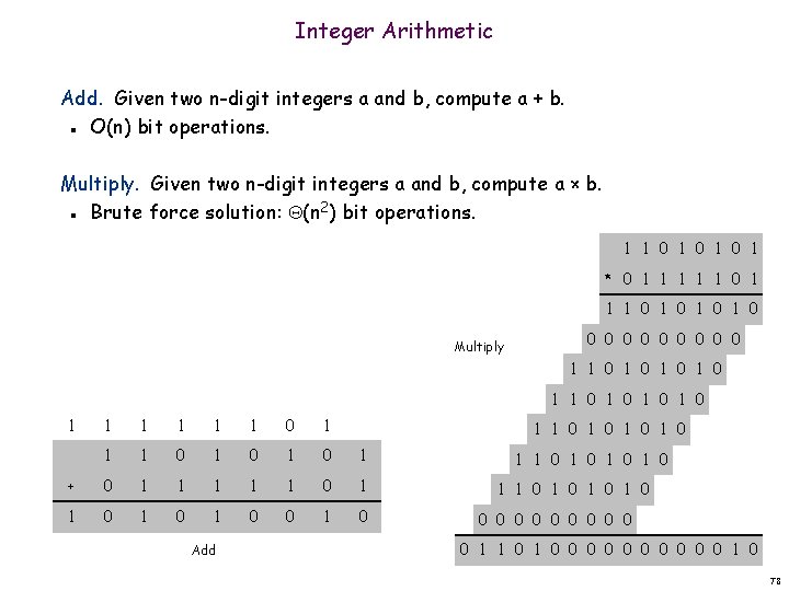
Integer Arithmetic Add. Given two n-digit integers a and b, compute a + b. O(n) bit operations. n Multiply. Given two n-digit integers a and b, compute a × b. Brute force solution: (n 2) bit operations. n 1 1 0 1 0 1 * 0 1 1 1 0 1 0 Multiply 0 0 0 0 0 1 1 0 1 0 1 1 1 0 1 0 1 + 0 1 1 1 0 1 0 1 0 Add 1 1 0 1 0 1 1 0 1 0 0 0 0 0 0 1 0 78
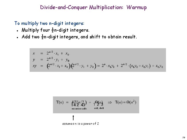
Divide-and-Conquer Multiplication: Warmup To multiply two n-digit integers: Multiply four ½n-digit integers. Add two ½n-digit integers, and shift to obtain result. n n assumes n is a power of 2 79
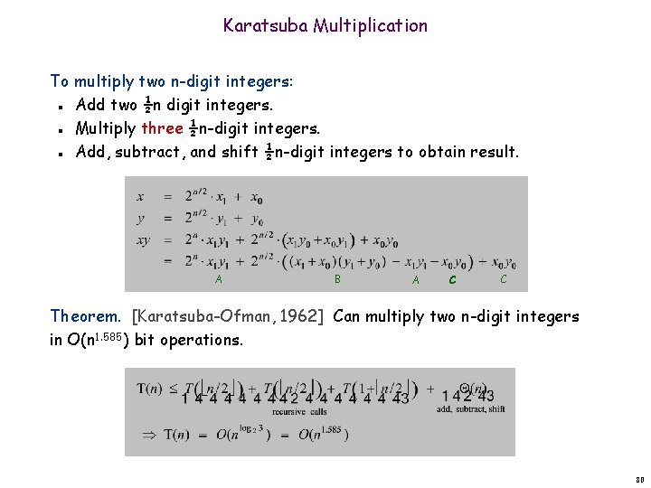
Karatsuba Multiplication To multiply two n-digit integers: Add two ½n digit integers. Multiply three ½n-digit integers. Add, subtract, and shift ½n-digit integers to obtain result. n n n A B A C C Theorem. [Karatsuba-Ofman, 1962] Can multiply two n-digit integers in O(n 1. 585) bit operations. 80
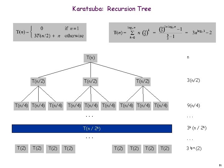
Karatsuba: Recursion Tree n T(n) T(n/2) 3(n/2) T(n/4) T(n/4) T(n/4) 9(n/4) . . . 3 k (n / 2 k) T(n / 2 k) . . . T(2) T(2) 3 lg n (2) 81
Matrix Multiplication
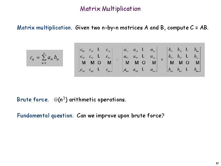
Matrix Multiplication Matrix multiplication. Given two n-by-n matrices A and B, compute C = AB. Brute force. (n 3) arithmetic operations. Fundamental question. Can we improve upon brute force? 83
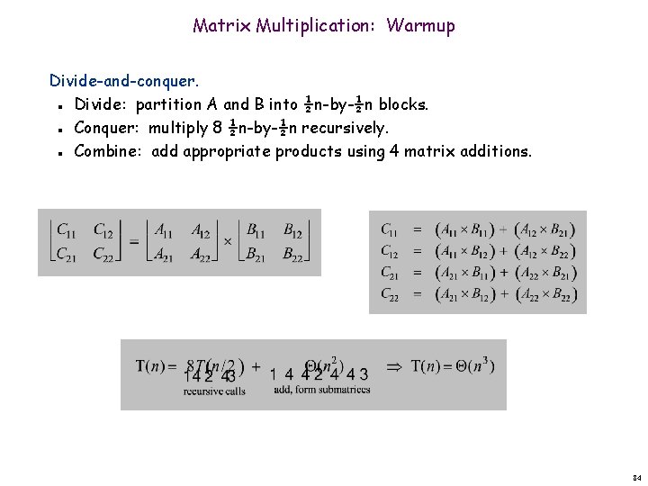
Matrix Multiplication: Warmup Divide-and-conquer. Divide: partition A and B into ½n-by-½n blocks. Conquer: multiply 8 ½n-by-½n recursively. Combine: add appropriate products using 4 matrix additions. n n n 84
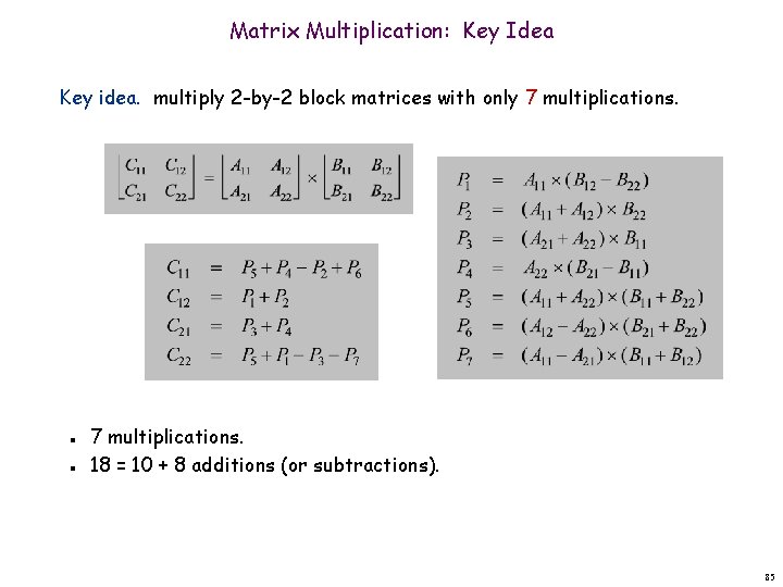
Matrix Multiplication: Key Idea Key idea. multiply 2 -by-2 block matrices with only 7 multiplications. n n 7 multiplications. 18 = 10 + 8 additions (or subtractions). 85
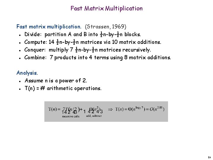
Fast Matrix Multiplication Fast matrix multiplication. (Strassen, 1969) Divide: partition A and B into ½n-by-½n blocks. Compute: 14 ½n-by-½n matrices via 10 matrix additions. Conquer: multiply 7 ½n-by-½n matrices recursively. Combine: 7 products into 4 terms using 8 matrix additions. n n Analysis. Assume n is a power of 2. T(n) = # arithmetic operations. n n 86

Fast Matrix Multiplication in Practice Implementation issues. Sparsity. Caching effects. Numerical stability. Odd matrix dimensions. Crossover to classical algorithm around n = 128. n n n Common misperception: "Strassen is only a theoretical curiosity. " Advanced Computation Group at Apple Computer reports 8 x speedup on G 4 Velocity Engine when n ~ 2, 500. Range of instances where it's useful is a subject of controversy. n n Remark. Can "Strassenize" Ax=b, determinant, eigenvalues, and other matrix ops. 87
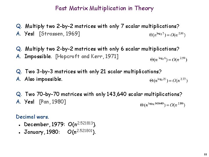
Fast Matrix Multiplication in Theory Q. Multiply two 2 -by-2 matrices with only 7 scalar multiplications? A. Yes! [Strassen, 1969] Q. Multiply two 2 -by-2 matrices with only 6 scalar multiplications? A. Impossible. [Hopcroft and Kerr, 1971] Q. Two 3 -by-3 matrices with only 21 scalar multiplications? A. Also impossible. Q. Two 70 -by-70 matrices with only 143, 640 scalar multiplications? A. Yes! [Pan, 1980] Decimal wars. December, 1979: O(n 2. 521813). January, 1980: O(n 2. 521801). n n 88
![Fast Matrix Multiplication in Theory Best known. O(n 2. 376) [Coppersmith-Winograd, 1987. ] Conjecture. Fast Matrix Multiplication in Theory Best known. O(n 2. 376) [Coppersmith-Winograd, 1987. ] Conjecture.](http://slidetodoc.com/presentation_image_h2/fd20ffb51f9745660af0278313113a89/image-89.jpg)
Fast Matrix Multiplication in Theory Best known. O(n 2. 376) [Coppersmith-Winograd, 1987. ] Conjecture. O(n 2+ ) for any > 0. Caveat. Theoretical improvements to Strassen are progressively less practical. 89
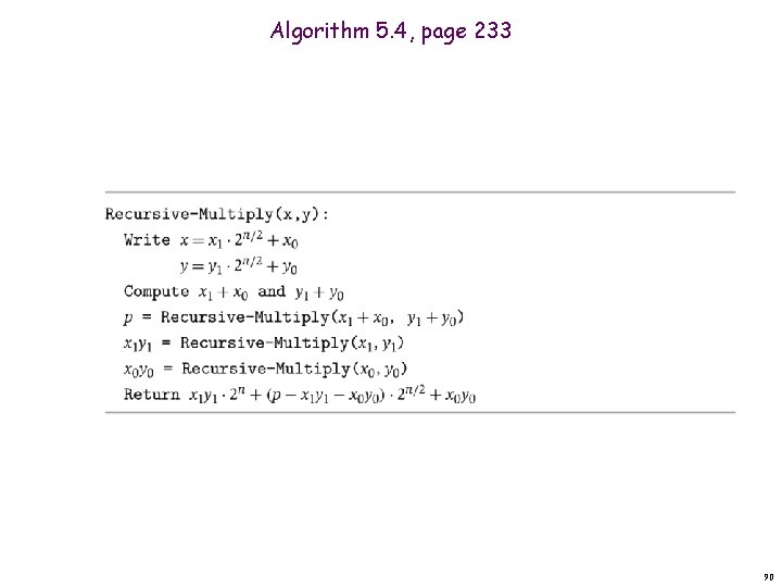
Algorithm 5. 4, page 233 90
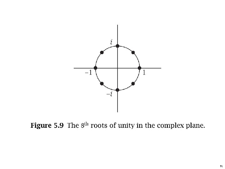
91
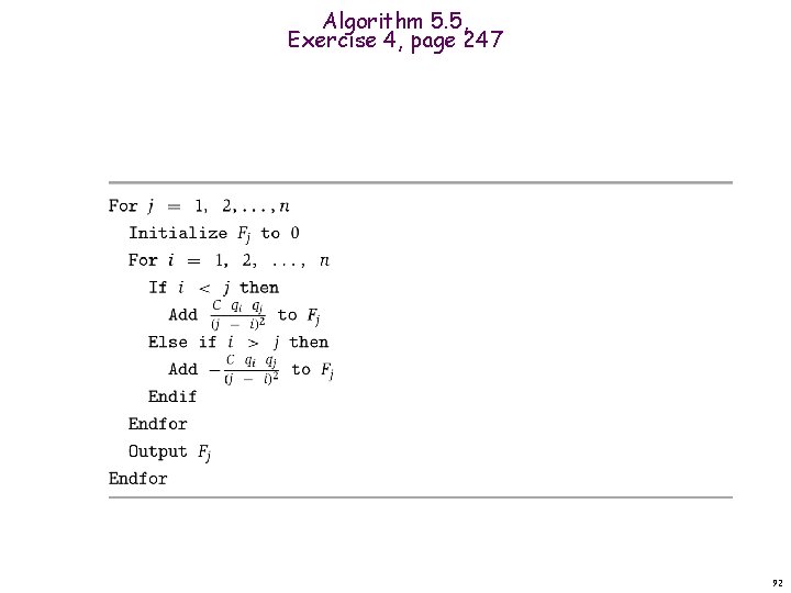
Algorithm 5. 5, Exercise 4, page 247 92
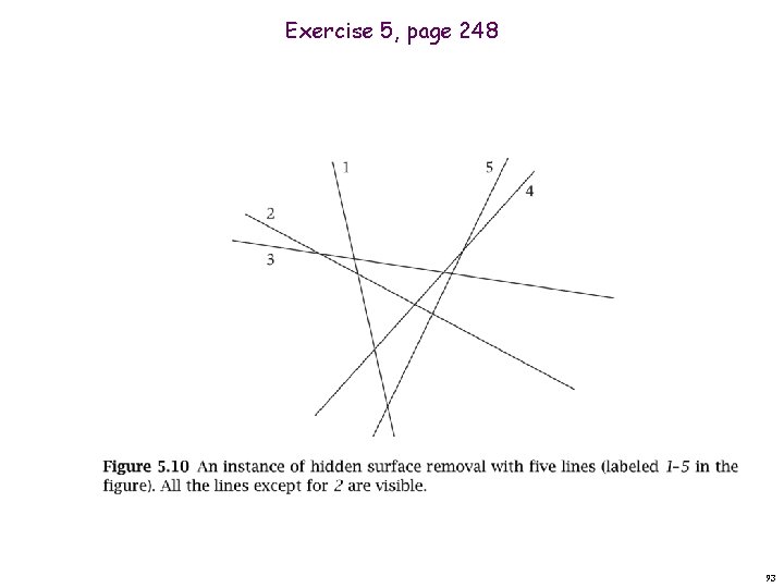
Exercise 5, page 248 93
- Slides: 93