Chapter 5 Discrete Random Variables C 5 L

Chapter 5 Discrete Random Variables C 5, L 1, S 1

Crown and Anchor Example • Pay $10 to play each game. • In one game, how much can I expect to win? Ie, if I played the game a very large number of times, how much would I win per game on average? C 5, L 1, S 2
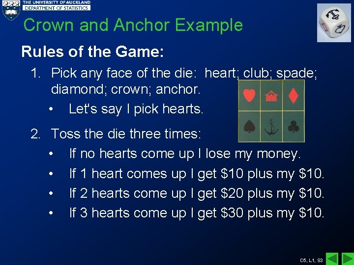
Crown and Anchor Example Rules of the Game: 1. Pick any face of the die: heart; club; spade; diamond; crown; anchor. • Let's say I pick hearts. 2. Toss the die three times: • If no hearts come up I lose my money. • If 1 heart comes up I get $10 plus my $10. • If 2 hearts come up I get $20 plus my $10. • If 3 hearts come up I get $30 plus my $10. C 5, L 1, S 3
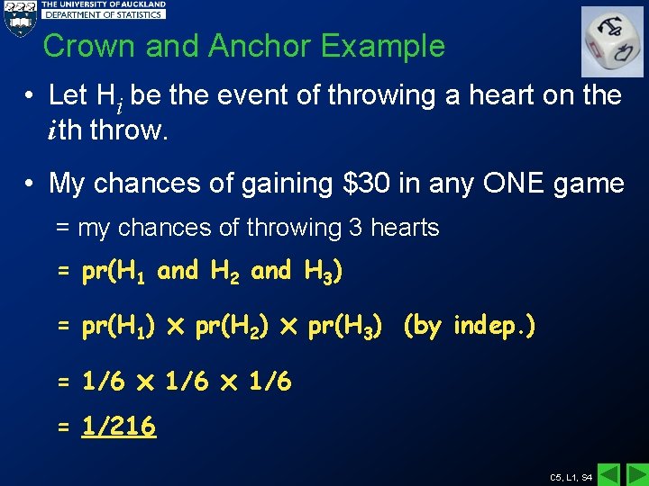
Crown and Anchor Example • Let Hi be the event of throwing a heart on the i th throw. • My chances of gaining $30 in any ONE game = my chances of throwing 3 hearts = pr(H 1 and H 2 and H 3) = pr(H 1) = 1/6 pr(H 2) 1/6 pr(H 3) (by indep. ) 1/6 = 1/216 C 5, L 1, S 4
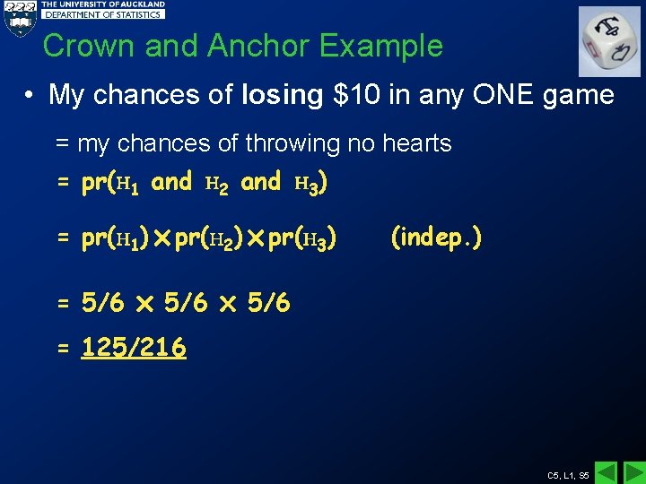
Crown and Anchor Example • My chances of losing $10 in any ONE game = my chances of throwing no hearts = pr(H 1 and H 2 and H 3) = pr(H 1) pr(H 2) pr(H 3) = 5/6 (indep. ) 5/6 = 125/216 C 5, L 1, S 5
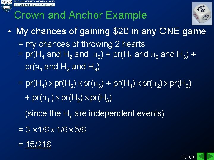
Crown and Anchor Example • My chances of gaining $20 in any ONE game = my chances of throwing 2 hearts = pr(H 1 and H 2 and H 3) + pr(H 1 and H 2 and H 3) = pr(H 1) pr(H 2) pr(H 3) + pr(H 1 ) pr(H 2) pr(H 3) (since the Hi are independent events) = 3 1/6 5/6 = 15/216 C 5, L 1, S 6

Crown and Anchor Example • My chances of gaining $10 in any ONE game = my chances of throwing 1 heart = pr(H 1 and H 2 and H 3) + pr(H 1 and H 2 and H 3) = pr(H 1) pr(H 2) pr(H 3) + pr(H 1) pr(H 2) pr(H 3) (since the Hi are independent events) = 3 1/6 5/6 = 75 / 216 C 5, L 1, S 7
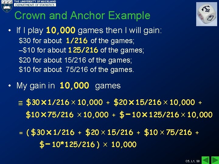
Crown and Anchor Example • If I play 10, 000 games then I will gain: $30 for about 1/216 of the games; –$10 for about 125/216 of the games; $20 for about 15/216 of the games; $10 for about 75/216 of the games. • My gain in 10, 000 games $30 1/216 10, 000 + $20 15/216 10, 000 + $10 75/216 10, 000 + $ -10 125/216 10, 000 = ( $30 1/216 + $20 15/216 + $10 75/216 + $ -10*125/216 ) 10, 000 C 5, L 1, S 8
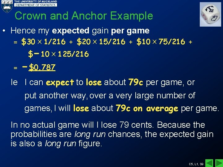
Crown and Anchor Example • Hence my expected gain per game = $30 1/216 + $20 15/216 + $10 75/216 + $ = -10 125/216 -$0. 787 Ie I can expect to lose about 79 c per game, or put another way, over a very large number of games, I will lose about 79 c on average per game. In no actual game will I lose 79 cents. Because the probabilities are long run chances, the expected gain is also a long run figure. C 5, L 1, S 9
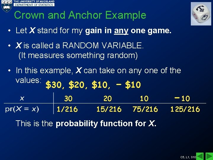
Crown and Anchor Example • Let X stand for my gain in any one game. • X is called a RANDOM VARIABLE. (It measures something random) • In this example, X can take on any one of the values: $30, $20, $10, - $10 30 1/216 20 15/216 10 75/216 -10 125/216 This is the probability function for X. C 5, L 1, S 10
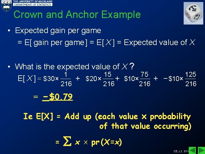
Crown and Anchor Example • Expected gain per game = E[ gain per game ] = E[ X ] = Expected value of X • What is the expected value of X ? 1 15 75 125 = + + + $20 $10 E[ X ] $30 216 = -$0. 79 216 216 Ie E[X] = Add up (each value probability of that value occurring) = x pr (X=x) C 5, L 1, S 11
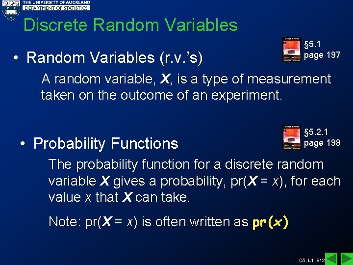
Discrete Random Variables • Random Variables (r. v. ’s) § 5. 1 page 197 A random variable, X, is a type of measurement taken on the outcome of an experiment. • Probability Functions § 5. 2. 1 page 198 The probability function for a discrete random variable X gives a probability, pr(X = x), for each value x that X can take. Note: pr(X = x) is often written as pr (x ) C 5, L 1, S 12
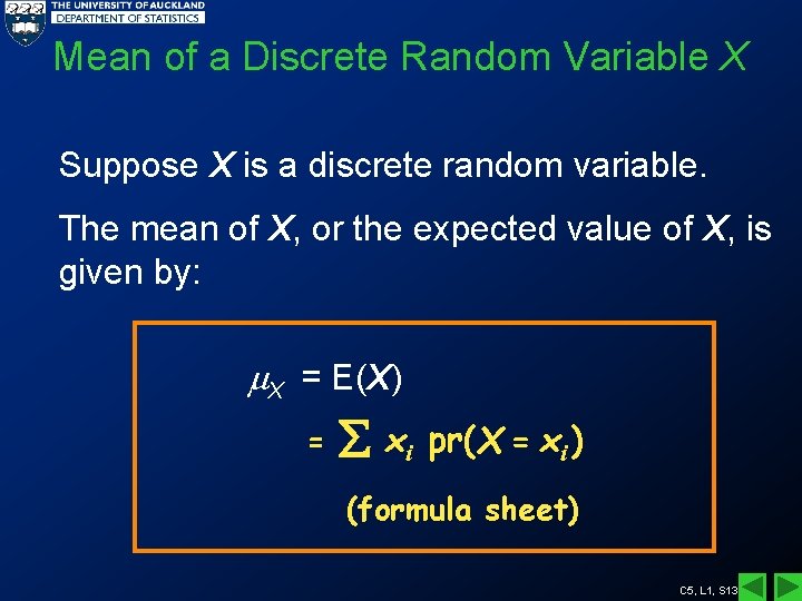
Mean of a Discrete Random Variable X Suppose X is a discrete random variable. The mean of X, or the expected value of X, is given by: X = E(X) = xi pr(X = xi ) (formula sheet) C 5, L 1, S 13
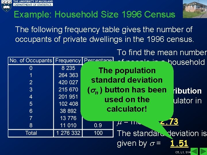
Example: Household Size 1996 Census The following frequency table gives the number of occupants of private dwellings in the 1996 census. To find the mean number of people in a household The population based on the standard deviation corresponding ( n ) button has been frequency distribution used the weon use our calculator in calculator! statistics mode. = mean = 2. 73 The standard deviation is given by = 1. 51 C 5, L 1, S 14
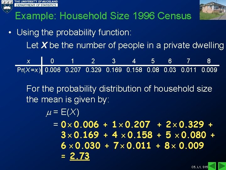
Example: Household Size 1996 Census • Using the probability function: Let X be the number of people in a private dwelling x 0 1 2 3 4 5 6 7 8 Pr(X =x ) 0. 006 0. 207 0. 329 0. 169 0. 158 0. 03 0. 011 0. 009 For the probability distribution of household size the mean is given by: = E(X ) = 0 0. 006 + 1 0. 207 + 2 0. 329 + 3 0. 169 + 4 0. 158 + 5 0. 080 + 6 0. 030 + 7 0. 011 + 8 0. 009 = 2. 73 C 5, L 1, S 15
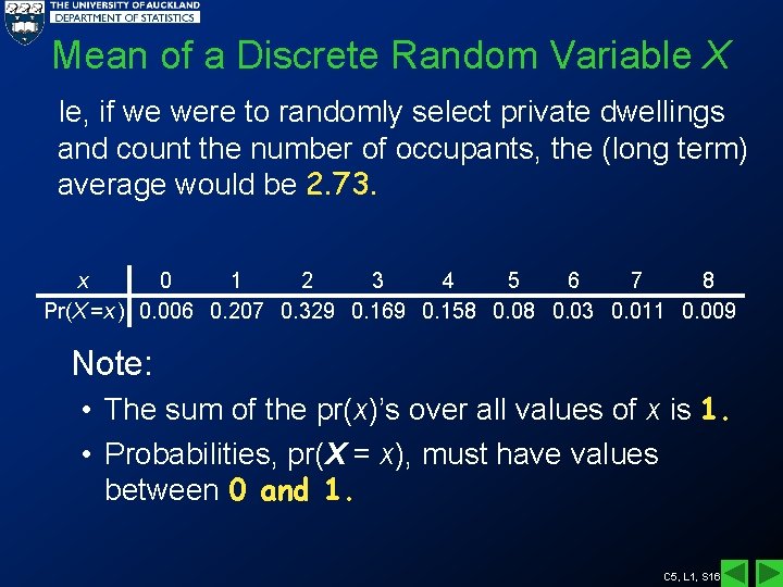
Mean of a Discrete Random Variable X Ie, if we were to randomly select private dwellings and count the number of occupants, the (long term) average would be 2. 73. x 0 1 2 3 4 5 6 7 8 Pr(X =x ) 0. 006 0. 207 0. 329 0. 169 0. 158 0. 03 0. 011 0. 009 Note: • The sum of the pr(x)’s over all values of x is 1. • Probabilities, pr(X = x), must have values between 0 and 1. C 5, L 1, S 16
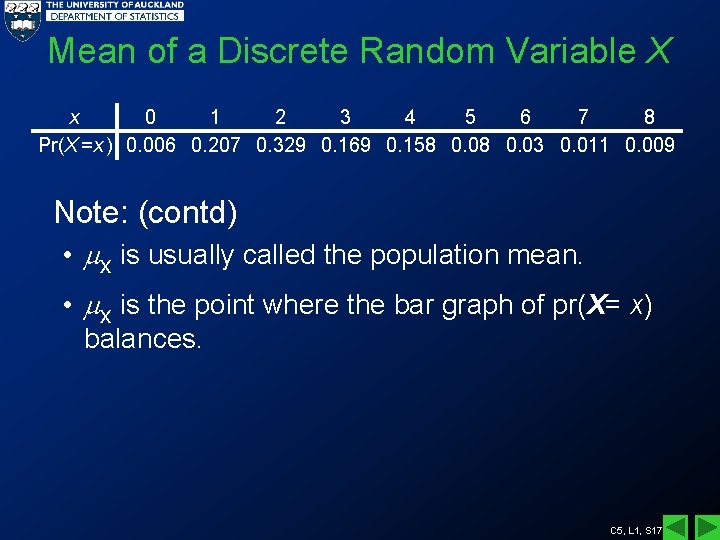
Mean of a Discrete Random Variable X x 0 1 2 3 4 5 6 7 8 Pr(X =x ) 0. 006 0. 207 0. 329 0. 169 0. 158 0. 03 0. 011 0. 009 Note: (contd) • x is usually called the population mean. • x is the point where the bar graph of pr(X= x) balances. C 5, L 1, S 17
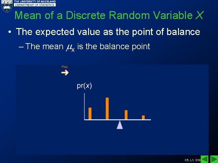
Mean of a Discrete Random Variable X • The expected value as the point of balance – The mean x is the balance point C 5, L 1, S 18
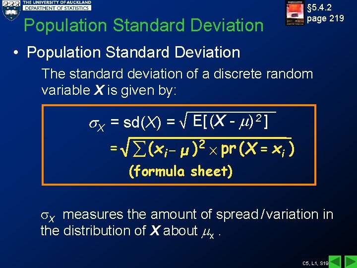
Population Standard Deviation § 5. 4. 2 page 219 • Population Standard Deviation The standard deviation of a discrete random variable X is given by: X = sd(X) = = E[ (X - ) 2 ] å (xi - μ )2 pr (X = xi ) (formula sheet) X measures the amount of spread / variation in the distribution of X about x. C 5, L 1, S 19
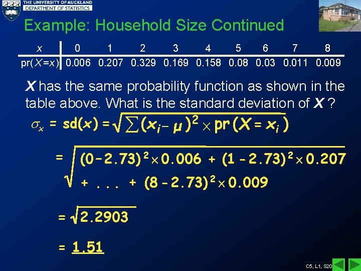
Example: Household Size Continued x 0 1 2 3 4 5 6 7 8 pr(X =x ) 0. 006 0. 207 0. 329 0. 169 0. 158 0. 03 0. 011 0. 009 X has the same probability function as shown in the table above. What is the standard deviation of X ? x = sd(x ) = å (x i - μ )2 pr (X = xi ) = (0 – 2. 73) 2 0. 006 + (1 - 2. 73) 2 0. 207 +. . . + (8 - 2. 73) 2 0. 009 = 2. 2903 = 1. 51 C 5, L 1, S 20
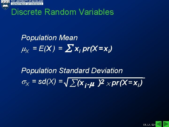
Discrete Random Variables Population Mean X = E(X ) = xi pr(X = xi ) Population Standard Deviation X = sd(X) = å (x -m )2 pr (X = xi ) i C 5, L 1, S 21
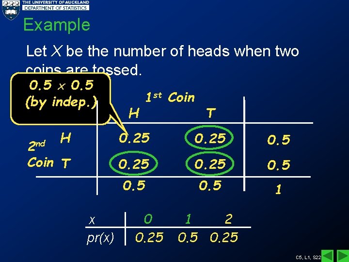
Example Let X be the number of heads when two coins are tossed. 0. 5 (by indep. ) H 1 st Coin T H 0. 25 0. 5 Coin T 0. 25 0. 5 1 2 nd x pr(x) 0 0. 25 1 2 0. 5 0. 25 C 5, L 1, S 22
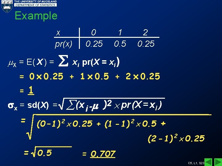
Example x pr(x) X = E( X ) = 0 0. 25 1 0. 5 2 0. 25 xi pr(X = xi ) = 0 0. 25 + 1 0. 5 + 2 0. 25 = 1 sx = sd(X) = å (x i -m )2 pr (X = xi ) = (0 – 1) 2 0. 25 + (1 - 1) 2 0. 5 + (2 - 1) 2 0. 25 = 0. 707 C 5, L 1, S 23
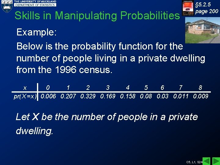
Skills in Manipulating Probabilities § 5. 2. 5 page 200 Example: Below is the probability function for the number of people living in a private dwelling from the 1996 census. x 0 1 2 3 4 5 6 7 8 pr(X =x ) 0. 006 0. 207 0. 329 0. 169 0. 158 0. 03 0. 011 0. 009 Let X be the number of people in a private dwelling. C 5, L 1, S 24
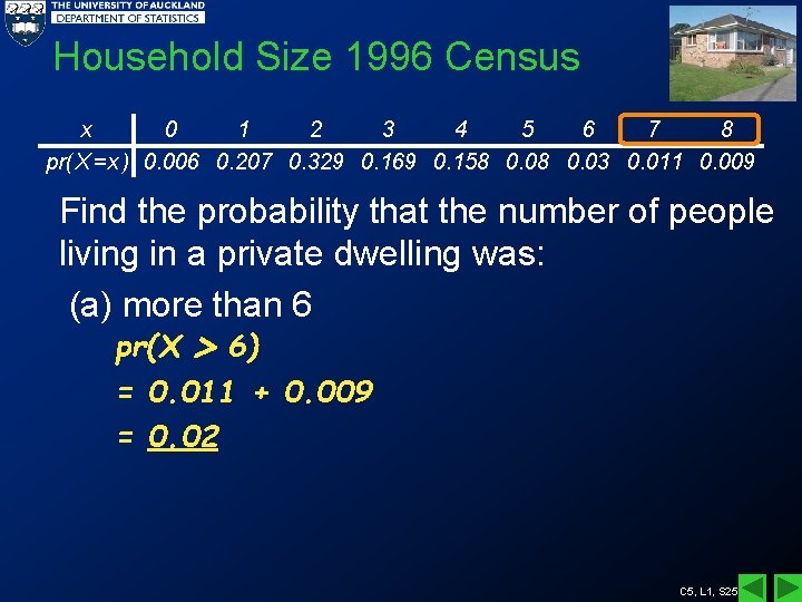
Household Size 1996 Census x 0 1 2 3 4 5 6 7 8 pr(X =x ) 0. 006 0. 207 0. 329 0. 169 0. 158 0. 03 0. 011 0. 009 Find the probability that the number of people living in a private dwelling was: (a) more than 6 pr(X 6) = 0. 011 + 0. 009 = 0. 02 C 5, L 1, S 25
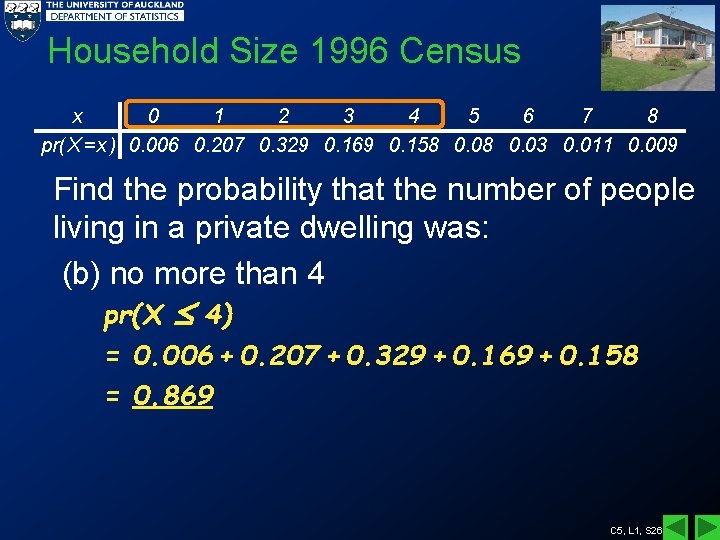
Household Size 1996 Census x 0 1 2 3 4 5 6 7 8 pr(X =x ) 0. 006 0. 207 0. 329 0. 169 0. 158 0. 03 0. 011 0. 009 Find the probability that the number of people living in a private dwelling was: (b) no more than 4 pr(X 4) = 0. 006 + 0. 207 + 0. 329 + 0. 169 + 0. 158 = 0. 869 C 5, L 1, S 26
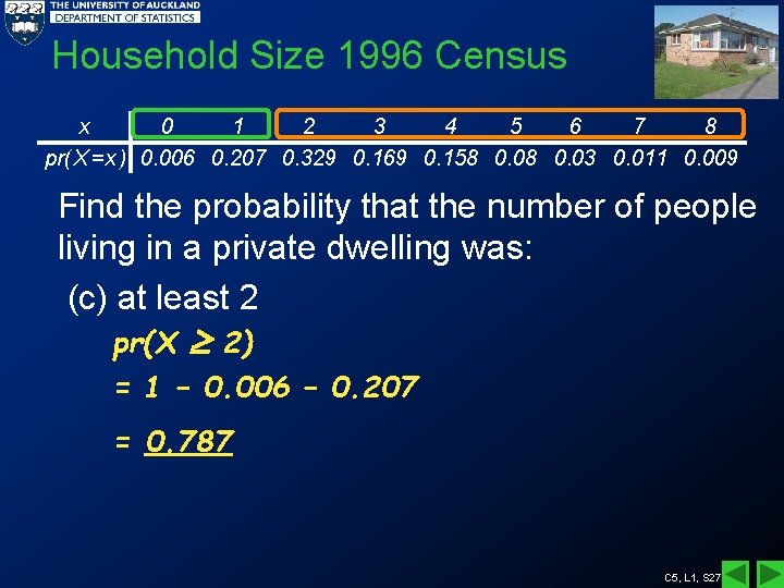
Household Size 1996 Census x 0 1 2 3 4 5 6 7 8 pr(X =x ) 0. 006 0. 207 0. 329 0. 169 0. 158 0. 03 0. 011 0. 009 Find the probability that the number of people living in a private dwelling was: (c) at least 2 pr(X 2) = 1 – 0. 006 – 0. 207 = 0. 787 C 5, L 1, S 27
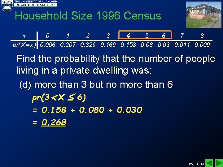
Household Size 1996 Census x 0 1 2 3 4 5 6 7 8 pr(X =x ) 0. 006 0. 207 0. 329 0. 169 0. 158 0. 03 0. 011 0. 009 Find the probability that the number of people living in a private dwelling was: (d) more than 3 but no more than 6 pr(3 X 6) = 0. 158 + 0. 080 + 0. 030 = 0. 268 C 5, L 1, S 28
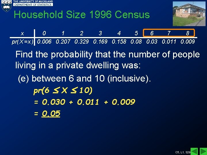
Household Size 1996 Census x 0 1 2 3 4 5 6 7 8 pr(X =x ) 0. 006 0. 207 0. 329 0. 169 0. 158 0. 03 0. 011 0. 009 Find the probability that the number of people living in a private dwelling was: (e) between 6 and 10 (inclusive). pr(6 X 10) = 0. 030 + 0. 011 + 0. 009 = 0. 05 C 5, L 1, S 29
• See: Example 5. 2. 5, page 200 • Try: Exercises § 5. 2, page 203 • Read: Taking care with language page 201 C 5, L 1, S 30
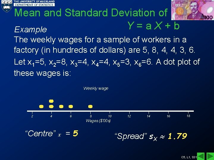
Mean and Standard Deviation of Y=a. X+b Example The weekly wages for a sample of workers in a factory (in hundreds of dollars) are 5, 8, 4, 4, 3, 6. Let x 1=5, x 2=8, x 3=4, x 4=4, x 5=3, x 6=6. A dot plot of these wages is: Weekly wage 2 4 6 8 10 12 14 16 18 Wages ($'00 s) “Centre” x = 5 “Spread” s. X 1. 79 C 5, L 1, S 31
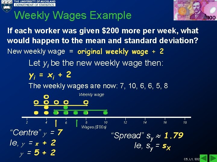
Weekly Wages Example If each worker was given $200 more per week, what would happen to the mean and standard deviation? New weekly wage = original weekly wage + 2 Let yi be the new weekly wage then: y i = xi + 2 The weekly wages are now: 7, 10, 6, 6, 5, 8 Weekly wage 2 4 “Centre” y = 7 Ie, y = x + 2 y =5+ 2 6 8 10 Wages ($'00 s) 12 14 16 18 “Spread” sy 1. 79 Ie, sy = s. X C 5, L 1, S 32
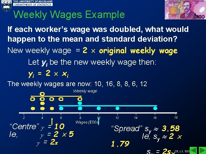
Weekly Wages Example If each worker’s wage was doubled, what would happen to the mean and standard deviation? New weekly wage = 2 original weekly wage Let yi be the new weekly wage then: y i = 2 xi The weekly wages are now: 10, 16, 8, 8, 6, 12 Weekly wage 2 4 6 “Centre” y = 10 Ie, y =2 5 y = 2 x 8 10 Wages ($'00 s) 12 14 16 18 “Spread” sy 3. 58 Ie, sy 2 1. 79 C 5, L 1, S 33
Weekly Wages Example If the manager gave a Christmas bonus of double the worker’s weekly wage plus $100 for extra spending, what would happen to the mean and standard deviation? Bonus = 2 original weekly wage + 1 Let yi be the bonus. y i = 2 xi + 1 The bonuses are: 11, 17, 9, 9, 7, 13 C 5, L 1, S 34
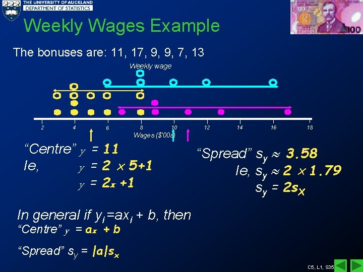
Weekly Wages Example The bonuses are: 11, 17, 9, 9, 7, 13 Weekly wage 2 4 6 8 10 12 14 16 18 Wages ($'00 s) “Centre” y = 11 Ie, y = 2 5+1 y = 2 x +1 “Spread” sy 3. 58 Ie, sy 2 1. 79 sy = 2 s. X In general if yi =axi + b, then “Centre” y = ax + b “Spread” sy = |a|sx C 5, L 1, S 35
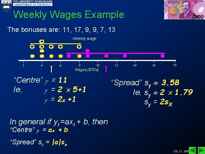
Weekly Wages Example The bonuses are: 11, 17, 9, 9, 7, 13 Weekly wage 2 4 6 8 10 12 14 16 18 Wages ($'00 s) “Centre” y = 11 Ie, y = 2 5+1 y = 2 x +1 “Spread” sy 3. 58 Ie, sy 2 1. 79 sy = 2 s. X In general if yi =axi + b, then “Centre” y = ax + b “Spread” sy = |a|sx C 5, L 1, S 36
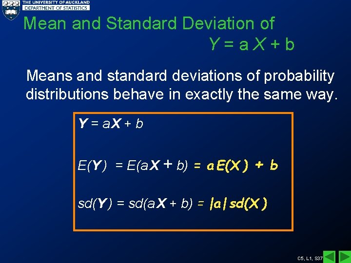
Mean and Standard Deviation of Y=a. X+b Means and standard deviations of probability distributions behave in exactly the same way. Y = a. X + b E(Y ) = E(a X + b) = a E(X ) + b sd(Y ) = sd(a X + b) = |a| sd(X ) C 5, L 1, S 37
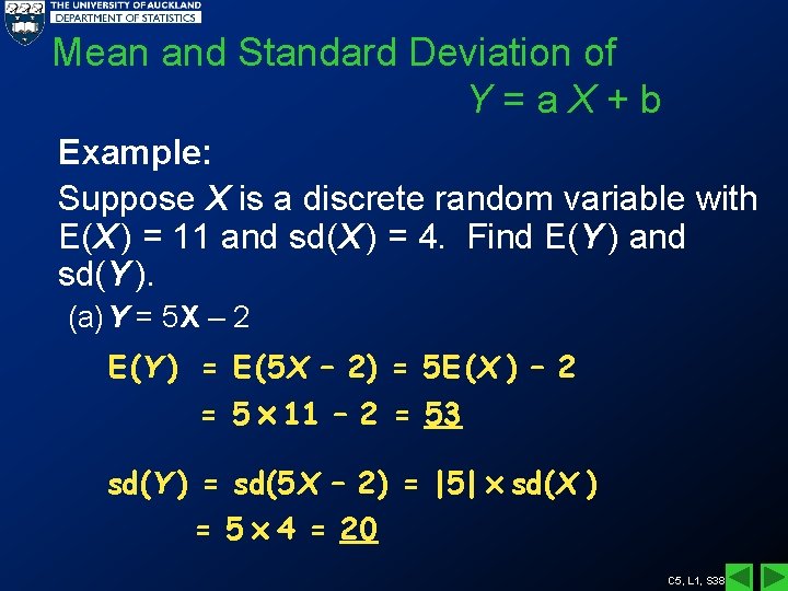
Mean and Standard Deviation of Y=a. X+b Example: Suppose X is a discrete random variable with E(X ) = 11 and sd(X ) = 4. Find E(Y ) and sd(Y ). (a)Y = 5 X – 2 E (Y ) = E (5 X – 2) = 5 E (X ) – 2 = 5 11 – 2 = 53 sd(Y ) = sd(5 X – 2) = |5| sd(X ) = 5 4 = 20 C 5, L 1, S 38
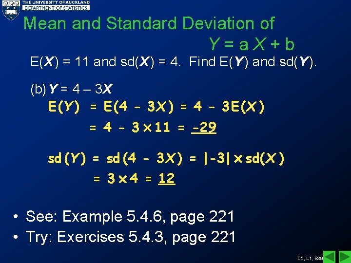
Mean and Standard Deviation of Y=a. X+b E(X ) = 11 and sd(X ) = 4. Find E(Y ) and sd(Y ). (b)Y = 4 – 3 X E (Y ) = E (4 - 3 X ) = 4 - 3 E (X ) = 4 - 3 11 = -29 sd (Y ) = sd (4 - 3 X ) = |-3| sd(X ) = 3 4 = 12 • See: Example 5. 4. 6, page 221 • Try: Exercises 5. 4. 3, page 221 C 5, L 1, S 39
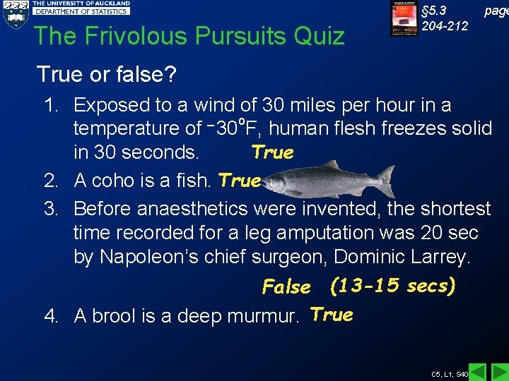
The Frivolous Pursuits Quiz § 5. 3 204 -212 page True or false? 1. Exposed to a wind of 30 miles per hour in a temperature of – 30 o. F, human flesh freezes solid in 30 seconds. True 2. A coho is a fish. True 3. Before anaesthetics were invented, the shortest time recorded for a leg amputation was 20 sec by Napoleon’s chief surgeon, Dominic Larrey. False (13 -15 secs) 4. A brool is a deep murmur. True C 5, L 1, S 40
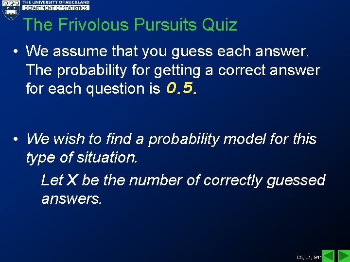
The Frivolous Pursuits Quiz • We assume that you guess each answer. The probability for getting a correct answer for each question is 0. 5. • We wish to find a probability model for this type of situation. Let X be the number of correctly guessed answers. C 5, L 1, S 41
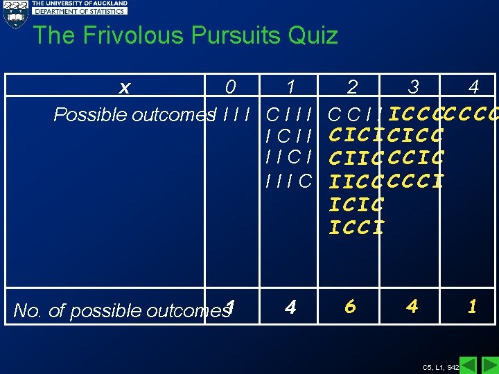
The Frivolous Pursuits Quiz x 0 1 Possible outcomes. I I C I ICII IICI IIIC No. of possible outcomes 1 4 2 3 4 C C I I I C C C C CICICICC CIIC CCIC IICCCCCI ICIC ICCI 6 4 1 C 5, L 1, S 42
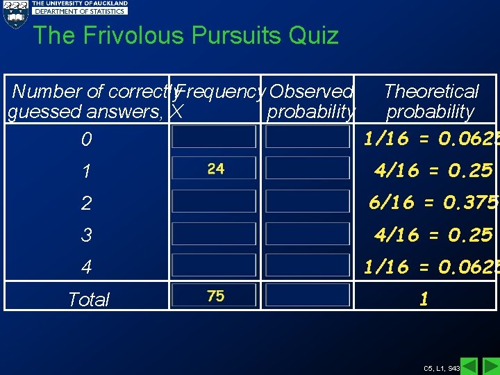
The Frivolous Pursuits Quiz Theoretical Number of correctly. Frequency Observed guessed answers, X probability 1/16 = 0. 0625 0 1 4/16 = 0. 25 2 6/16 = 0. 375 3 4/16 = 0. 25 4 1/16 = 0. 0625 Total 1 C 5, L 1, S 43
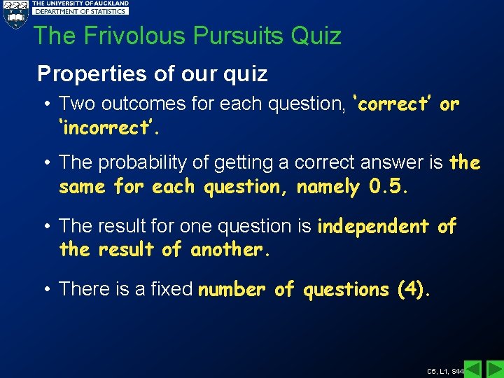
The Frivolous Pursuits Quiz Properties of our quiz • Two outcomes for each question, ‘correct’ or ‘incorrect’. • The probability of getting a correct answer is the same for each question, namely 0. 5. • The result for one question is independent of the result of another. • There is a fixed number of questions (4). C 5, L 1, S 44
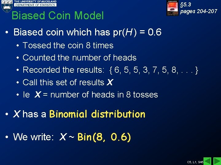
Biased Coin Model § 5. 3 pages 204 -207 • Biased coin which has pr(H ) = 0. 6 • • • Tossed the coin 8 times Counted the number of heads Recorded the results: { 6, 5, 5, 3, 7, 5, 8, . . . } Call this set of results X Ie X = number of heads in 8 tosses • X has a Binomial distribution • We write: X ~ Bin (8, 0. 6) C 5, L 1, S 45
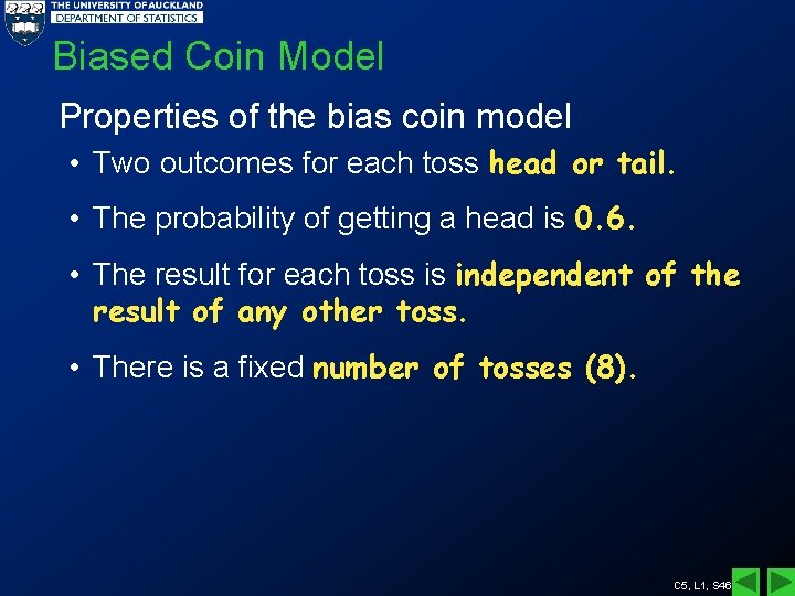
Biased Coin Model Properties of the bias coin model • Two outcomes for each toss head or tail. • The probability of getting a head is 0. 6. • The result for each toss is independent of the result of any other toss. • There is a fixed number of tosses (8). C 5, L 1, S 46
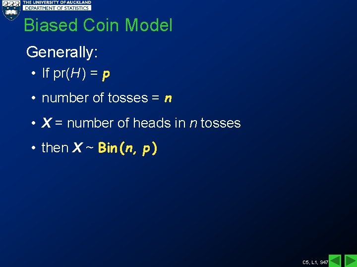
Biased Coin Model Generally: • If pr(H ) = p • number of tosses = n • X = number of heads in n tosses • then X ~ Bin (n, p ) C 5, L 1, S 47
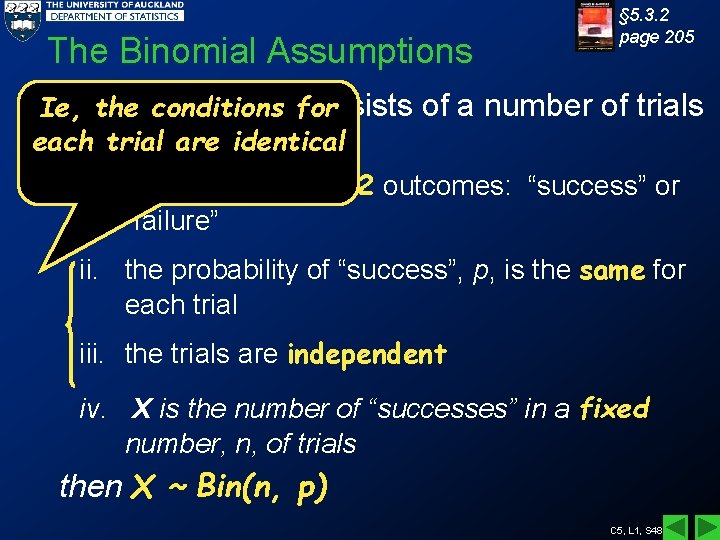
The Binomial Assumptions § 5. 3. 2 page 205 If an consists of a number of trials Ie, theexperiment conditions for each andtrial are identical i. each trial has only 2 outcomes: “success” or “failure” ii. the probability of “success”, p, is the same for each trial iii. the trials are independent iv. X is the number of “successes” in a fixed number, n, of trials then X ~ Bin(n, p) C 5, L 1, S 48
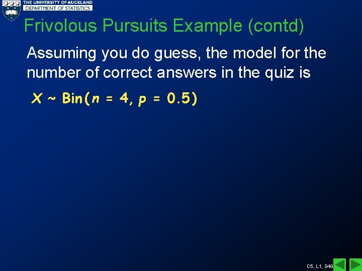
Frivolous Pursuits Example (contd) Assuming you do guess, the model for the number of correct answers in the quiz is X ~ Bin ( n = 4, p = 0. 5 ) C 5, L 1, S 49
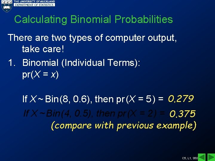
Calculating Binomial Probabilities There are two types of computer output, take care! 1. Binomial (Individual Terms): pr(X = x) If X ~ Bin (8, 0. 6), then pr (X = 5 ) = 0. 279 If X ~ Bin (4, 0. 5), then pr (X = 2 ) = 0. 375 (compare with previous example) C 5, L 1, S 50
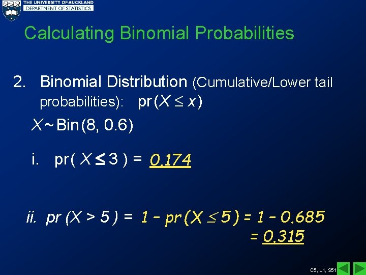
Calculating Binomial Probabilities 2. Binomial Distribution (Cumulative/Lower tail probabilities): pr (X x ) X ~ Bin (8, 0. 6 ) i. pr ( X 3 ) = 0. 174 ii. pr (X > 5 ) = 1 – pr (X 5 ) = 1 – 0. 685 = 0. 315 C 5, L 1, S 51
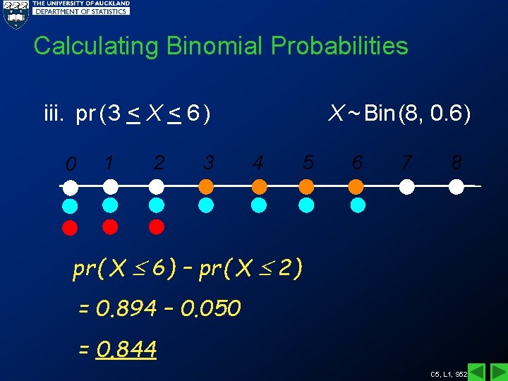
Calculating Binomial Probabilities iii. pr ( 3 < X < 6 ) 0 1 2 3 X ~ Bin (8, 0. 6 ) 4 5 6 7 8 pr ( X 6 ) – pr ( X 2 ) = 0. 894 – 0. 050 = 0. 844 C 5, L 1, S 52
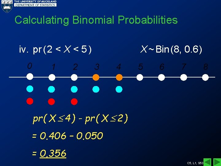
Calculating Binomial Probabilities iv. pr ( 2 < X < 5 ) 0 1 2 X ~ Bin (8, 0. 6 ) 3 4 5 6 7 8 pr ( X 4 ) - pr ( X 2 ) = 0. 406 – 0. 050 = 0. 356 C 5, L 1, S 53
Calculating Binomial Probabilities Note: Using the Binomial tables and formula to find probabilities is non-examinable material. Computer output will be provided for tests and exams. See: How to use MINITAB and Excel to page 207 produce probabilities C 5, L 1, S 54
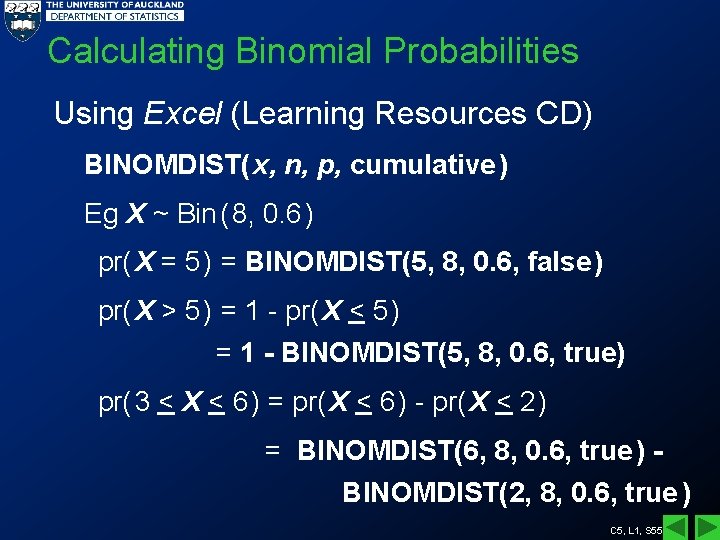
Calculating Binomial Probabilities Using Excel (Learning Resources CD) BINOMDIST( x, n, p, cumulative ) Eg X ~ Bin ( 8, 0. 6 ) pr( X = 5 ) = BINOMDIST(5, 8, 0. 6, false ) pr( X > 5 ) = 1 - pr( X < 5 ) = 1 - BINOMDIST(5, 8, 0. 6, true) pr( 3 < X < 6 ) = pr( X < 6 ) - pr( X < 2 ) = BINOMDIST(6, 8, 0. 6, true ) BINOMDIST(2, 8, 0. 6, true ) C 5, L 1, S 55
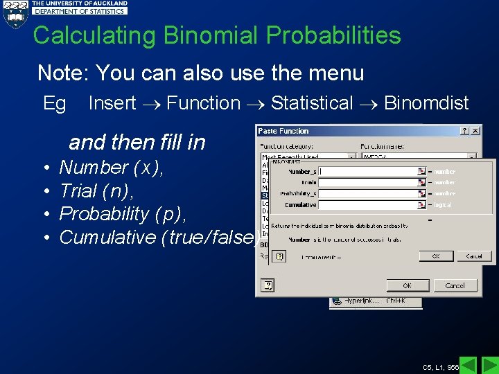
Calculating Binomial Probabilities Note: You can also use the menu Eg Insert Function Statistical Binomdist and then fill in • • Number ( x ), Trial ( n ), Probability ( p ), Cumulative ( true / false ) C 5, L 1, S 56
Sampling Without Replacement § 5. 3. 3 page 210 If we take a sample of size n from a much larger population in which a proportion p have a characteristic of interest, the distribution of X, the number in the sample with that characteristic, is approximately Binomial (n, p). Operating rule: Approximation is adequate if n < 0. 1 N where N is the population size. C 5, L 1, S 57
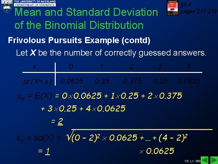
Mean and Standard Deviation of the Binomial Distribution § 5. 4 pages 217 -219 Frivolous Pursuits Example (contd) Let X be the number of correctly guessed answers. x pr ( X= x ) 0 1 2 3 4 0. 0625 0. 375 0. 25 0. 0625 X = E(X ) = 0 0. 0625 + 1 0. 25 + 2 0. 375 + 3 0. 25 + 4 0. 0625 =2 s. X = sd(X) = (0 – 2)2 0. 0625 + … + (4 – 2)2 =1 0. 0625 C 5, L 1, S 58
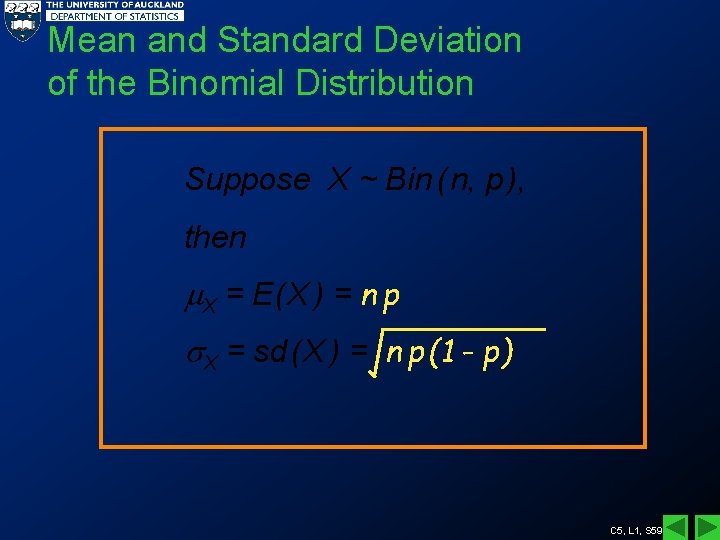
Mean and Standard Deviation of the Binomial Distribution Suppose X ~ Bin ( n, p ), then X = E( X ) = n p X = sd ( X ) = n p (1 - p) C 5, L 1, S 59
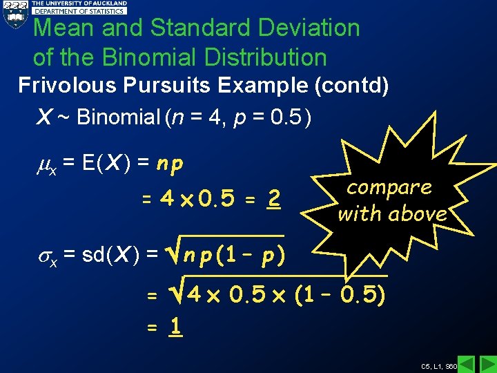
Mean and Standard Deviation of the Binomial Distribution Frivolous Pursuits Example (contd) X ~ Binomial (n = 4, p = 0. 5 ) x = E( X ) = n p = 4 0. 5 = 2 compare with above x = sd( X ) = n p (1 – p ) = 4 0. 5 (1 – 0. 5) = 1 C 5, L 1, S 60
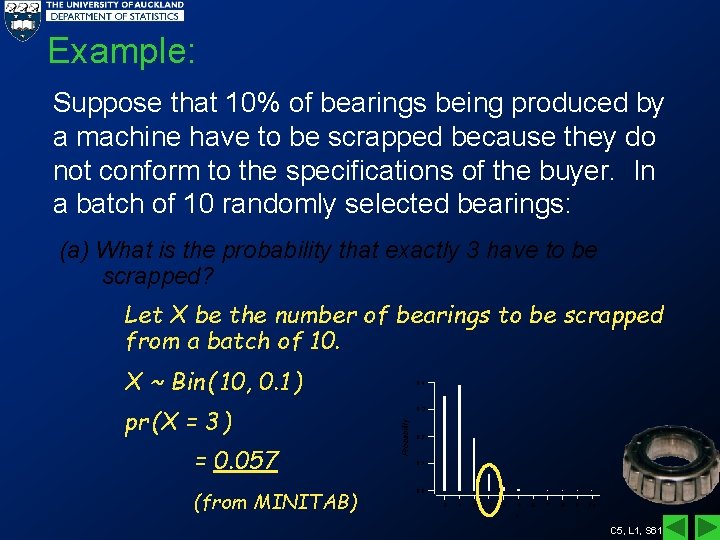
Example: Suppose that 10% of bearings being produced by a machine have to be scrapped because they do not conform to the specifications of the buyer. In a batch of 10 randomly selected bearings: (a) What is the probability that exactly 3 have to be scrapped? Let X be the number of bearings to be scrapped from a batch of 10. X ~ Bin ( 10, 0. 1 ) = 0. 057 (from MINITAB) 0. 3 Probability pr (X = 3 ) 0. 4 0. 2 0. 1 0. 0 0 1 2 3 4 5 6 7 8 9 10 x C 5, L 1, S 61
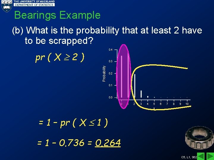
Bearings Example (b) What is the probability that at least 2 have to be scrapped? pr ( X 2 ) = 1 – pr ( X 1 ) = 1 – 0. 736 = 0. 264 C 5, L 1, S 62
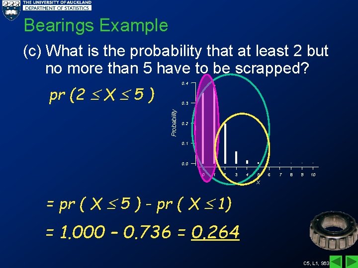
Bearings Example (c) What is the probability that at least 2 but no more than 5 have to be scrapped? 0. 4 pr (2 X 5 ) Probability 0. 3 0. 2 0. 1 0. 0 0 1 2 3 4 5 6 7 8 9 10 x = pr ( X 5 ) - pr ( X 1) = 1. 000 – 0. 736 = 0. 264 C 5, L 1, S 63
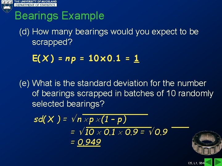
Bearings Example (d) How many bearings would you expect to be scrapped? E( X ) = n p = 10 0. 1 = 1 (e) What is the standard deviation for the number of bearings scrapped in batches of 10 randomly selected bearings? sd( X ) = n p (1 – p ) = 10 0. 1 0. 9 = 0. 949 C 5, L 1, S 64
The Poisson Distribution Example: An office receives, on average, 18 phone calls per hour. Count the number of calls received in one hour. On one occasion there were 13 calls in one hour. On another occasion there were 22 calls in one hour, and so on. Let X be the number of phone calls per hour. Under certain conditions we can say X has a Poisson (18) distribution. Ie X ~ Poisson (18). C 5, L 1, S 65
The Poisson Distribution More Examples: X is the number of: • errors in a given set of accounts • scratches on a CD surface • bacterial colonies in 2 litres of milk Ie X is the number of occurrences in a given time / space under certain conditions. C 5, L 1, S 66
The Poisson Distribution Conditions: 1. The events occur at a constant average rate of (lambda) per unit time / space. 2. Occurrences are independent of one another. 3. The probability of 2 or more occurrences in a time / space interval of size d approaches 0 as d approaches 0. Ie occurrences don’t happen at exactly the same time / space. C 5, L 1, S 67
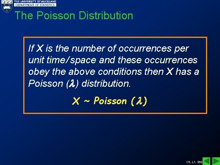
The Poisson Distribution If X is the number of occurrences per unit time / space and these occurrences obey the above conditions then X has a Poisson ( ) distribution. X ~ Poisson ( ) C 5, L 1, S 68
The Poisson Distribution Notes: i. is the parameter for this distribution. (Where a parameter is a numerical characteristic of the population). ii. In this course it will not be necessary to use the formula for the Poisson probability function or tables. Computer output of pr(X = x) (individual terms) and pr(X x) (cumulative/lower tails) are given in tests and exams. C 5, L 1, S 69
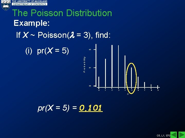
The Poisson Distribution Example: If X ~ Poisson( = 3), find: (i) pr(X = 5) P r o b a b ilit y 0. 2 0. 1 0. 0 0 1 2 3 4 5 6 7 8 9 X pr(X = 5) = 0. 101 C 5, L 1, S 70
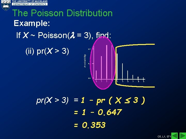
The Poisson Distribution Example: If X ~ Poisson( = 3), find: P ro b a b ility (ii) pr(X > 3) 0. 2 0. 1 0. 0 0 1 2 3 4 5 6 7 8 9 X pr(X > 3) = 1 – pr ( X 3 ) = 1 – 0. 647 = 0. 353 C 5, L 1, S 71
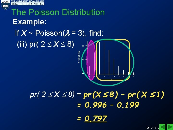
The Poisson Distribution Example: If X ~ Poisson( = 3), find: (iii) pr( 2 X 8) P ro b a b ility 0. 2 0. 1 0. 0 0 1 2 3 4 5 6 7 8 9 X pr( 2 X 8) = pr (X 8 ) – pr ( X 1) = 0. 996 – 0. 199 = 0. 797 C 5, L 1, S 72
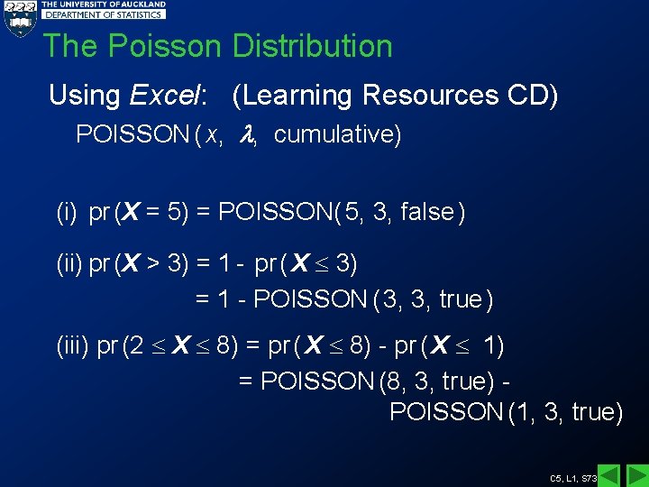
The Poisson Distribution Using Excel: (Learning Resources CD) POISSON ( x, , cumulative) (i) pr (X = 5) = POISSON( 5, 3, false ) (ii) pr (X > 3) = 1 - pr ( X 3) = 1 - POISSON ( 3, 3, true ) (iii) pr (2 X 8) = pr ( X 8) - pr ( X 1) = POISSON (8, 3, true) POISSON (1, 3, true) C 5, L 1, S 73
The Poisson Distribution Using MINITAB: (Learning Resources CD) • Look under Calc Probability Distributions Poisson • Choose probability for pr ( X = x ) and cumulative for pr ( X <= x ) • Fill in mean and input column C 5, L 1, S 74
The Poisson Distribution Example: Suppose a manufacturing company has a mean of 24 accidents per year. If the number of accidents per year is known to have a Poisson distribution, find the following probabilities. Let X be the number of accidents per month X ~ Poisson ( = 2 ) [ = 24/12 ] (i) There are no accidents in a given month. (ii) There at least 2 accidents in a given month. C 5, L 1, S 75
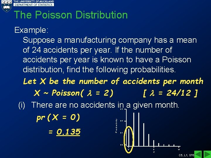
The Poisson Distribution Example: Suppose a manufacturing company has a mean of 24 accidents per year. If the number of accidents per year is known to have a Poisson distribution, find the following probabilities. Let X be the number of accidents per month X ~ Poisson ( = 2 ) [ = 24/12 ] (i) There are no accidents in a given month. pr ( X = 0 ) = 0. 135 P r o b a b ility 0. 3 0. 2 0. 1 0. 0 0 5 10 X C 5, L 1, S 76
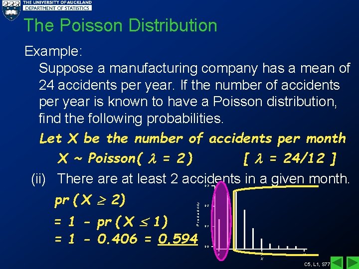
The Poisson Distribution Example: Suppose a manufacturing company has a mean of 24 accidents per year. If the number of accidents per year is known to have a Poisson distribution, find the following probabilities. Let X be the number of accidents per month X ~ Poisson ( = 2 ) [ = 24/12 ] (ii) There at least 2 accidents in a given month. pr ( X 2) P r o b a b ility 0. 3 = 1 - pr ( X 1) = 1 - 0. 406 = 0. 594 0. 2 0. 1 0. 0 0 5 10 X C 5, L 1, S 77
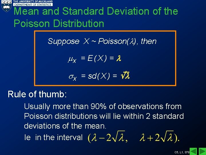
Mean and Standard Deviation of the Poisson Distribution Suppose X ~ Poisson( ), then X = E ( X ) = X = sd ( X ) = Rule of thumb: Usually more than 90% of observations from Poisson distributions will lie within 2 standard deviations of the mean. Ie in the interval C 5, L 1, S 78
Example 1 The Gainsville Sun (10 May 1980) reported that 18 employees of the nuclear weapons research facility, Lawrence Livermore Laboratory (California, U. S. A. ), contracted the deadly skin cancer melanoma during the period 1972 -77. In comparison, in the previous 20 -year period, the mean number of occurrences was 2. 3 cases per 5 -year period. If the mean rate of melanoma cases per 5 year period was 2. 3, should it be considered unusual that 18 cases have occurred in one 5 -year period? C 5, L 1, S 79
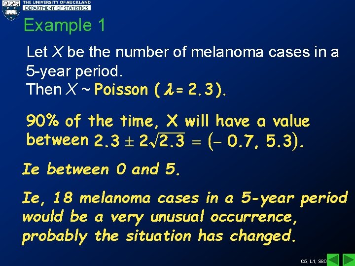
Example 1 Let X be the number of melanoma cases in a 5 -year period. Then X ~ Poisson ( = 2. 3 ). 90% of the time, X will have a value between Ie between 0 and 5. Ie, 18 melanoma cases in a 5 -year period would be a very unusual occurrence, probably the situation has changed. C 5, L 1, S 80
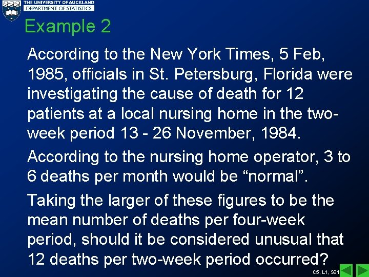
Example 2 According to the New York Times, 5 Feb, 1985, officials in St. Petersburg, Florida were investigating the cause of death for 12 patients at a local nursing home in the twoweek period 13 - 26 November, 1984. According to the nursing home operator, 3 to 6 deaths per month would be “normal”. Taking the larger of these figures to be the mean number of deaths per four-week period, should it be considered unusual that 12 deaths per two-week period occurred? C 5, L 1, S 81
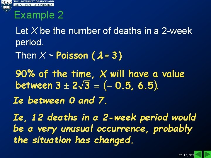
Example 2 Let X be the number of deaths in a 2 -week period. Then X ~ Poisson ( = 3 ) 90% of the time, X will have a value between Ie between 0 and 7. Ie, 12 deaths in a 2 -week period would be a very unusual occurrence, probably the situation has changed. C 5, L 1, S 82
Exercise Identify whether the following random variables can be modelled by either the Binomial or Poisson distribution. If they can, find the value / s of the parameter / s. C 5, L 1, S 83
Exercise a) In the long run, 80% of ACE light bulbs last for 1000 hrs of continuous operation. You need to have 20 lights in your attic for a small business enterprise, so you buy a batch of 20 light bulbs. Let X 1 be the number of these bulbs that have to be replaced by the time 1000 hrs are up. X 1 ~ Bin ( 20, 0. 2 ) C 5, L 1, S 84
Exercise b) In (a), because of the continual need for replacement bulbs, you buy a batch of 1000 cheap bulbs. Of these 100 have disconnected filaments. You start off by using 20 bulbs (which we assume are randomly chosen). Let X 2 be the number with disconnected filaments. X 2 ~ Bin (20, 0. 1) ( n / N = 20 / 1000 = 0. 02 < 0. 1) C 5, L 1, S 85
Exercise c) Suppose that telephone calls come into the university switchboard randomly at a rate of 100 per hour. Let X 3 be the number of calls in a 1 -hour period. X 3 ~ Poisson (100) C 5, L 1, S 86
Exercise d) In (c), 60% of callers know the extension number of the person they wish to call. Suppose 120 calls are received in a given hour. Let X 4 be the number of callers who know the extension number. X 4 ~ Bin ( 120, 0. 6 ) C 5, L 1, S 87
Exercise e) In (d), let X 5 be the number of calls taken up to and including the first call where the caller did not know the extension number. Neither. Not fixed no. of trials; not no. of occurrences per unit time / space. C 5, L 1, S 88
Exercise f) It so happened that of the 120 calls in (d), 70 callers knew the extension number and 50 did not. Assume calls go randomly to telephone operators. Suppose telephone operator A took 10 calls. Of the calls taken by operator A, let X 6 be the number made by callers who knew the extension number. X 6 ~ Bin ( 10, 70 / 120 ) (n / N = 10 / 120 = 0. 08 < 0. 1 ) C 5, L 1, S 89
Exercise g) Suppose heart attack victims come to a 200 -bed hospital at a rate of three per week on average. Let X 7 be the number of heart attack victims admitted in one week. X 7 ~ Poisson (3 ) C 5, L 1, S 90
Exercise h) Suppose 20 patients, of whom 9 had “flu”, came to a doctor’s surgery on a particular morning. The order of arrival was random as far as having flu was concerned. The doctor only had time to see 15 patients before lunch. Let X 8 be the number of flu patients seen before lunch. Neither. Not Binomial since n / N = 15 / 20 = 0. 75 which is not < 0. 1. C 5, L 1, S 91
Exercise i) Suppose meteor showers are arriving randomly at a rate of 40 per hour. Let X 9 be the number of showers arriving in a 15 -minute period. X 9 ~ Poisson (10 ) C 5, L 1, S 92
- Slides: 92