Chapter 5 DecreaseandConquer Design and Analysis of Algorithms

Chapter 5 Decrease-and-Conquer Design and Analysis of Algorithms - Chapter 5 Copyright © 2007 Pearson Addison-Wesley. All rights reserved.

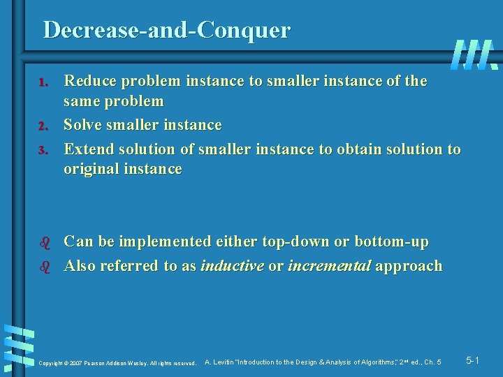
Decrease-and-Conquer 1. 2. 3. b b Reduce problem instance to smaller instance of the same problem Solve smaller instance Extend solution of smaller instance to obtain solution to original instance Can be implemented either top-down or bottom-up Also referred to as inductive or incremental approach Copyright © 2007 Pearson Addison-Wesley. All rights reserved. A. Levitin “Introduction to the Design & Analysis of Algorithms, ” 2 nd ed. , Ch. 5 5 -1

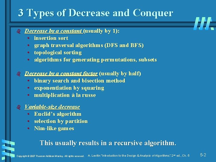
3 Types of Decrease and Conquer b Decrease by a constant (usually by 1): • insertion sort • graph traversal algorithms (DFS and BFS) • topological sorting • algorithms for generating permutations, subsets b Decrease by a constant factor (usually by half) • binary search and bisection method • exponentiation by squaring • multiplication à la russe b Variable-size decrease • Euclid’s algorithm • selection by partition • Nim-like games This usually results in a recursive algorithm. Copyright © 2007 Pearson Addison-Wesley. All rights reserved. A. Levitin “Introduction to the Design & Analysis of Algorithms, ” 2 nd ed. , Ch. 5 5 -2

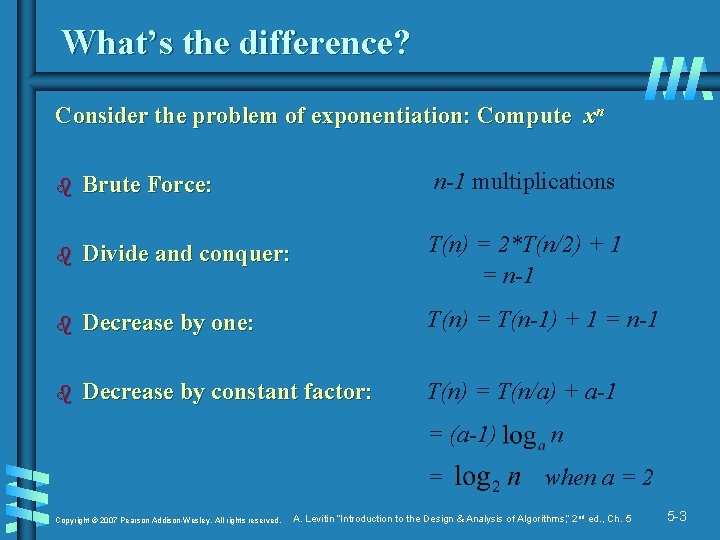
What’s the difference? Consider the problem of exponentiation: Compute xn b Brute Force: n-1 multiplications b Divide and conquer: T(n) = 2*T(n/2) + 1 = n-1 b Decrease by one: T(n) = T(n-1) + 1 = n-1 b Decrease by constant factor: T(n) = T(n/a) + a-1 Copyright © 2007 Pearson Addison-Wesley. All rights reserved. = (a-1) n = when a = 2 A. Levitin “Introduction to the Design & Analysis of Algorithms, ” 2 nd ed. , Ch. 5 5 -3

Insertion Sort To sort array A[0. . n-1], sort A[0. . n-2] recursively and then insert A[n-1] in its proper place among the sorted A[0. . n-2] b Usually implemented bottom up (nonrecursively) Example: Sort 6, 4, 1, 8, 5 6|4 1 8 5 4 6|1 8 5 1 4 6|8 5 1 4 6 8|5 1 4 5 6 8 Copyright © 2007 Pearson Addison-Wesley. All rights reserved. A. Levitin “Introduction to the Design & Analysis of Algorithms, ” 2 nd ed. , Ch. 5 5 -4

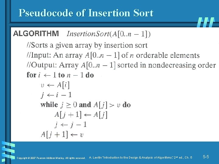
Pseudocode of Insertion Sort Copyright © 2007 Pearson Addison-Wesley. All rights reserved. A. Levitin “Introduction to the Design & Analysis of Algorithms, ” 2 nd ed. , Ch. 5 5 -5

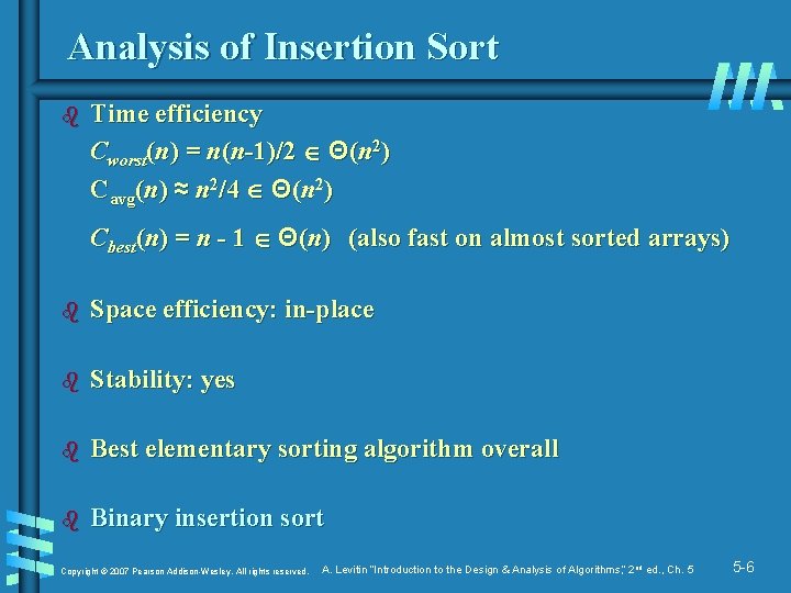
Analysis of Insertion Sort b Time efficiency Cworst(n) = n(n-1)/2 Θ(n 2) Cavg(n) ≈ n 2/4 Θ(n 2) Cbest(n) = n - 1 Θ(n) (also fast on almost sorted arrays) b Space efficiency: in-place b Stability: yes b Best elementary sorting algorithm overall b Binary insertion sort Copyright © 2007 Pearson Addison-Wesley. All rights reserved. A. Levitin “Introduction to the Design & Analysis of Algorithms, ” 2 nd ed. , Ch. 5 5 -6

Graph Traversal Many problems require processing all graph vertices (and edges) in systematic fashion Graph traversal algorithms: • Depth-first search (DFS) • Breadth-first search (BFS) Copyright © 2007 Pearson Addison-Wesley. All rights reserved. A. Levitin “Introduction to the Design & Analysis of Algorithms, ” 2 nd ed. , Ch. 5 5 -7

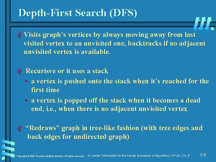
Depth-First Search (DFS) b Visits graph’s vertices by always moving away from last visited vertex to an unvisited one, backtracks if no adjacent unvisited vertex is available. b Recurisve or it uses a stack • a vertex is pushed onto the stack when it’s reached for the first time • a vertex is popped off the stack when it becomes a dead end, i. e. , when there is no adjacent unvisited vertex b “Redraws” graph in tree-like fashion (with tree edges and back edges for undirected graph) Copyright © 2007 Pearson Addison-Wesley. All rights reserved. A. Levitin “Introduction to the Design & Analysis of Algorithms, ” 2 nd ed. , Ch. 5 5 -8

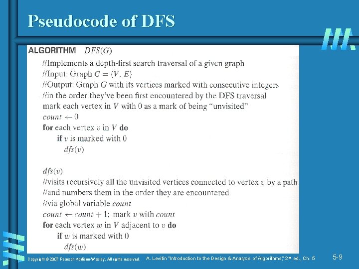
Pseudocode of DFS Copyright © 2007 Pearson Addison-Wesley. All rights reserved. A. Levitin “Introduction to the Design & Analysis of Algorithms, ” 2 nd ed. , Ch. 5 5 -9

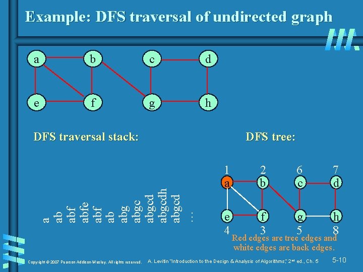
Example: DFS traversal of undirected graph a b c d e f g h DFS tree: a ab abfe abf ab abgcdh abgcd … DFS traversal stack: Copyright © 2007 Pearson Addison-Wesley. All rights reserved. 1 a 2 b 6 c e 4 f 3 g 5 7 d h 8 Red edges are tree edges and white edges are back edges. A. Levitin “Introduction to the Design & Analysis of Algorithms, ” 2 nd ed. , Ch. 5 5 -10

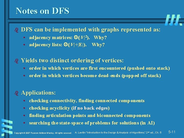
Notes on DFS b DFS can be implemented with graphs represented as: • adjacency matrices: Θ(|V|2). Why? • adjacency lists: Θ(|V|+|E|). Why? b Yields two distinct ordering of vertices: • order in which vertices are first encountered (pushed onto stack) • order in which vertices become dead-ends (popped off stack) b Applications: • • checking connectivity, finding connected components checking acyclicity (if no back edges) finding articulation points and biconnected components searching the state-space of problems for solutions (in AI) Copyright © 2007 Pearson Addison-Wesley. All rights reserved. A. Levitin “Introduction to the Design & Analysis of Algorithms, ” 2 nd ed. , Ch. 5 5 -11

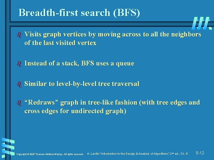
Breadth-first search (BFS) b Visits graph vertices by moving across to all the neighbors of the last visited vertex b Instead of a stack, BFS uses a queue b Similar to level-by-level tree traversal b “Redraws” graph in tree-like fashion (with tree edges and cross edges for undirected graph) Copyright © 2007 Pearson Addison-Wesley. All rights reserved. A. Levitin “Introduction to the Design & Analysis of Algorithms, ” 2 nd ed. , Ch. 5 5 -12

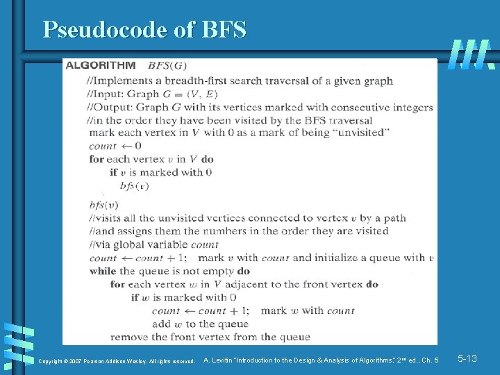
Pseudocode of BFS Copyright © 2007 Pearson Addison-Wesley. All rights reserved. A. Levitin “Introduction to the Design & Analysis of Algorithms, ” 2 nd ed. , Ch. 5 5 -13

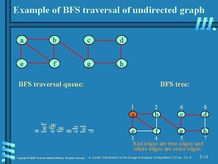
Example of BFS traversal of undirected graph a b c d e f g h BFS tree: a bef efg fg g ch hd d BFS traversal queue: 1 2 6 8 a b c d e f g h 3 4 5 7 Red edges are tree edges and white edges are cross edges. Copyright © 2007 Pearson Addison-Wesley. All rights reserved. A. Levitin “Introduction to the Design & Analysis of Algorithms, ” 2 nd ed. , Ch. 5 5 -14

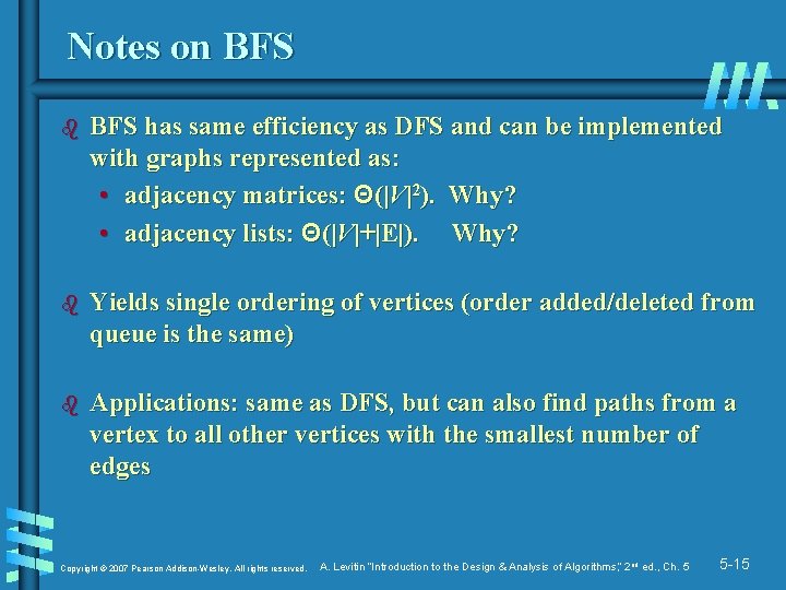
Notes on BFS b BFS has same efficiency as DFS and can be implemented with graphs represented as: • adjacency matrices: Θ(|V|2). Why? • adjacency lists: Θ(|V|+|E|). Why? b Yields single ordering of vertices (order added/deleted from queue is the same) b Applications: same as DFS, but can also find paths from a vertex to all other vertices with the smallest number of edges Copyright © 2007 Pearson Addison-Wesley. All rights reserved. A. Levitin “Introduction to the Design & Analysis of Algorithms, ” 2 nd ed. , Ch. 5 5 -15

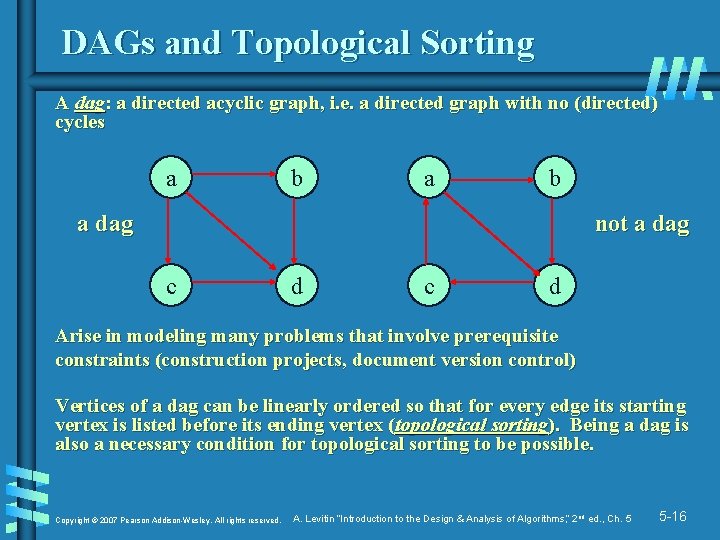
DAGs and Topological Sorting A dag: a directed acyclic graph, i. e. a directed graph with no (directed) cycles a b a dag not a dag c d Arise in modeling many problems that involve prerequisite constraints (construction projects, document version control) Vertices of a dag can be linearly ordered so that for every edge its starting vertex is listed before its ending vertex (topological sorting). Being a dag is also a necessary condition for topological sorting to be possible. Copyright © 2007 Pearson Addison-Wesley. All rights reserved. A. Levitin “Introduction to the Design & Analysis of Algorithms, ” 2 nd ed. , Ch. 5 5 -16

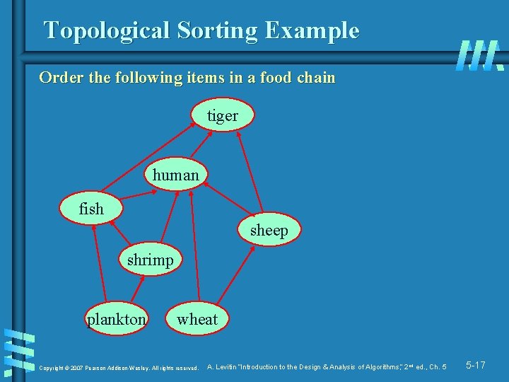
Topological Sorting Example Order the following items in a food chain tiger human fish sheep shrimp plankton wheat Copyright © 2007 Pearson Addison-Wesley. All rights reserved. A. Levitin “Introduction to the Design & Analysis of Algorithms, ” 2 nd ed. , Ch. 5 5 -17

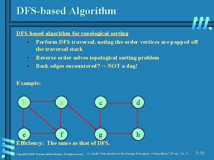
DFS-based Algorithm DFS-based algorithm for topological sorting • Perform DFS traversal, noting the order vertices are popped off the traversal stack • Reverse order solves topological sorting problem • Back edges encountered? → NOT a dag! Example: b a c d e f g h Efficiency: The same as that of DFS. Copyright © 2007 Pearson Addison-Wesley. All rights reserved. A. Levitin “Introduction to the Design & Analysis of Algorithms, ” 2 nd ed. , Ch. 5 5 -18

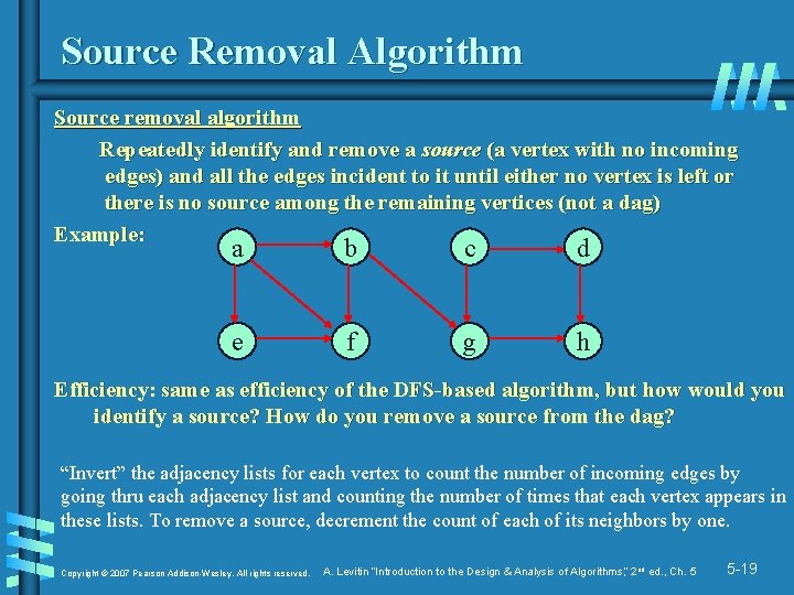
Source Removal Algorithm Source removal algorithm Repeatedly identify and remove a source (a vertex with no incoming edges) and all the edges incident to it until either no vertex is left or there is no source among the remaining vertices (not a dag) Example: a b c d e f g h Efficiency: same as efficiency of the DFS-based algorithm, but how would you identify a source? How do you remove a source from the dag? “Invert” the adjacency lists for each vertex to count the number of incoming edges by going thru each adjacency list and counting the number of times that each vertex appears in these lists. To remove a source, decrement the count of each of its neighbors by one. Copyright © 2007 Pearson Addison-Wesley. All rights reserved. A. Levitin “Introduction to the Design & Analysis of Algorithms, ” 2 nd ed. , Ch. 5 5 -19

Decrease-by-Constant-Factor Algorithms In this variation of decrease-and-conquer, instance size is reduced by the same factor (typically, 2) Examples: • Binary search and the method of bisection • Exponentiation by squaring • Multiplication à la russe (Russian peasant method) • Fake-coin puzzle • Josephus problem Copyright © 2007 Pearson Addison-Wesley. All rights reserved. A. Levitin “Introduction to the Design & Analysis of Algorithms, ” 2 nd ed. , Ch. 5 5 -20

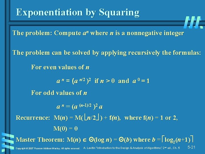
Exponentiation by Squaring The problem: Compute an where n is a nonnegative integer The problem can be solved by applying recursively the formulas: For even values of n a n = (a n/2 )2 if n > 0 and a 0 = 1 For odd values of n a n = (a (n-1)/2 )2 a Recurrence: M(n) = M( n/2 ) + f(n), where f(n) = 1 or 2, M(0) = 0 Master Theorem: M(n) Θ(log n) = Θ(b) where b = log 2(n+1) Copyright © 2007 Pearson Addison-Wesley. All rights reserved. A. Levitin “Introduction to the Design & Analysis of Algorithms, ” 2 nd ed. , Ch. 5 5 -21

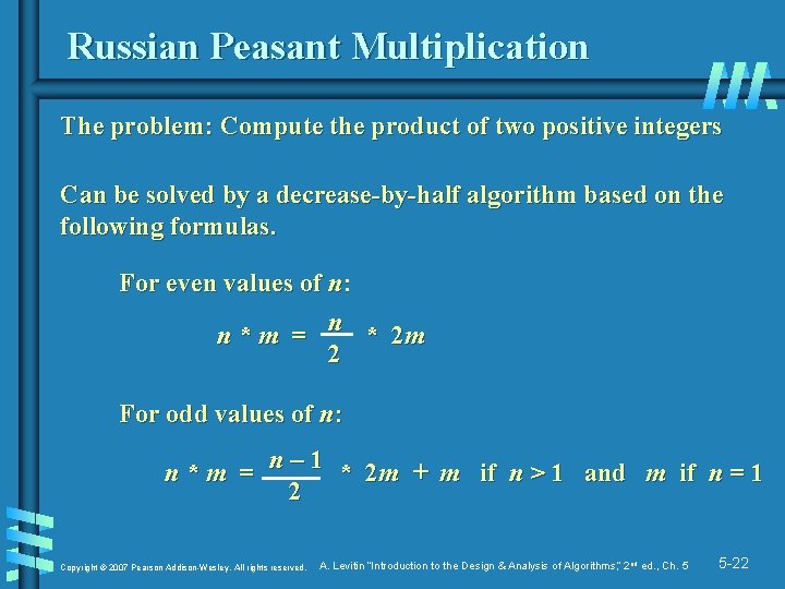
Russian Peasant Multiplication The problem: Compute the product of two positive integers Can be solved by a decrease-by-half algorithm based on the following formulas. For even values of n: n * m = n * 2 m 2 For odd values of n: n * m = n – 1 * 2 m + m if n > 1 and m if n = 1 2 Copyright © 2007 Pearson Addison-Wesley. All rights reserved. A. Levitin “Introduction to the Design & Analysis of Algorithms, ” 2 nd ed. , Ch. 5 5 -22

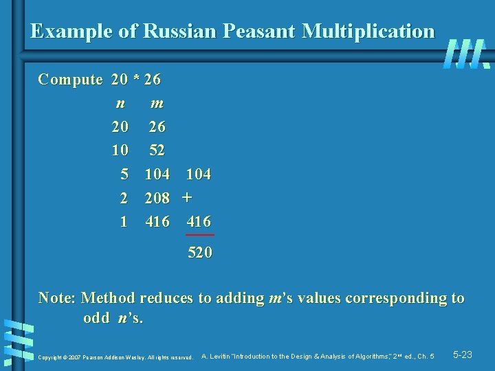
Example of Russian Peasant Multiplication Compute 20 * 26 n m 20 26 10 52 5 104 2 208 1 416 104 + 416 520 Note: Method reduces to adding m’s values corresponding to odd n’s. Copyright © 2007 Pearson Addison-Wesley. All rights reserved. A. Levitin “Introduction to the Design & Analysis of Algorithms, ” 2 nd ed. , Ch. 5 5 -23

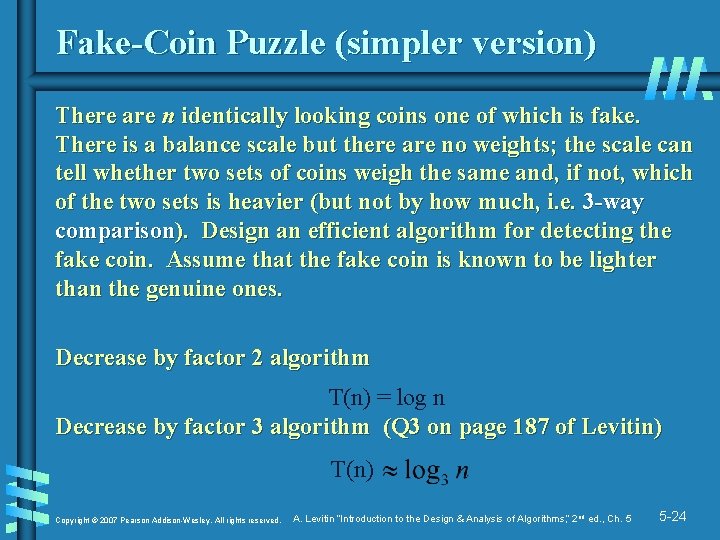
Fake-Coin Puzzle (simpler version) There are n identically looking coins one of which is fake. There is a balance scale but there are no weights; the scale can tell whether two sets of coins weigh the same and, if not, which of the two sets is heavier (but not by how much, i. e. 3 -way comparison). Design an efficient algorithm for detecting the fake coin. Assume that the fake coin is known to be lighter than the genuine ones. Decrease by factor 2 algorithm T(n) = log n Decrease by factor 3 algorithm (Q 3 on page 187 of Levitin) T(n) Copyright © 2007 Pearson Addison-Wesley. All rights reserved. A. Levitin “Introduction to the Design & Analysis of Algorithms, ” 2 nd ed. , Ch. 5 5 -24

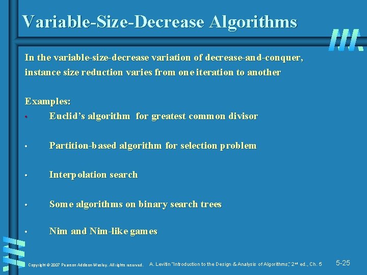
Variable-Size-Decrease Algorithms In the variable-size-decrease variation of decrease-and-conquer, instance size reduction varies from one iteration to another Examples: • Euclid’s algorithm for greatest common divisor • Partition-based algorithm for selection problem • Interpolation search • Some algorithms on binary search trees • Nim and Nim-like games Copyright © 2007 Pearson Addison-Wesley. All rights reserved. A. Levitin “Introduction to the Design & Analysis of Algorithms, ” 2 nd ed. , Ch. 5 5 -25

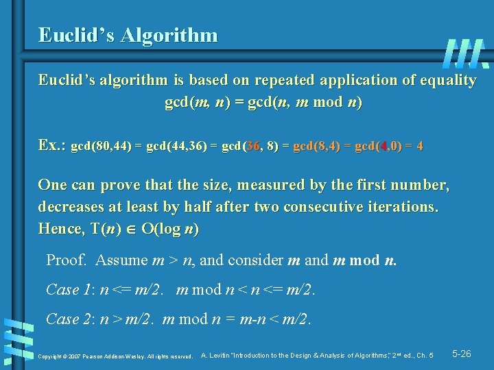
Euclid’s Algorithm Euclid’s algorithm is based on repeated application of equality gcd(m, n) = gcd(n, m mod n) Ex. : gcd(80, 44) = gcd(44, 36) = gcd(36, 8) = gcd(8, 4) = gcd(4, 0) = 4 One can prove that the size, measured by the first number, decreases at least by half after two consecutive iterations. Hence, T(n) O(log n) Proof. Assume m > n, and consider m and m mod n. Case 1: n <= m/2. m mod n <= m/2. Case 2: n > m/2. m mod n = m-n < m/2. Copyright © 2007 Pearson Addison-Wesley. All rights reserved. A. Levitin “Introduction to the Design & Analysis of Algorithms, ” 2 nd ed. , Ch. 5 5 -26

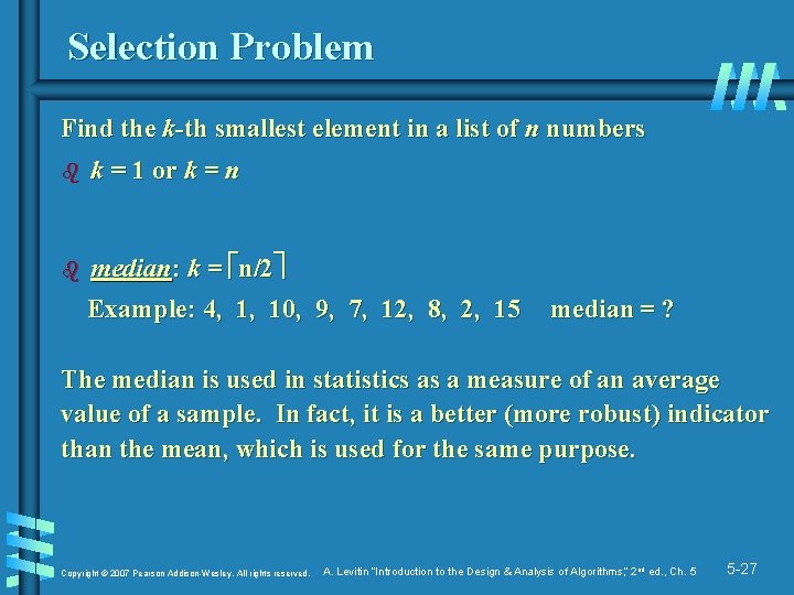
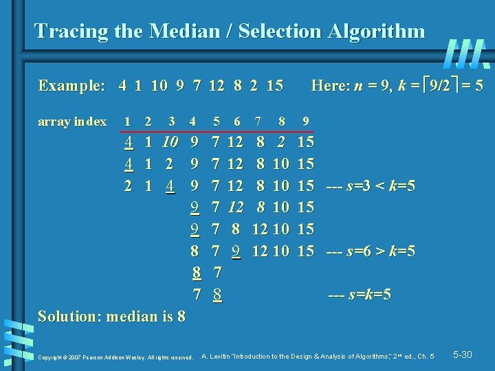
Selection Problem Find the k-th smallest element in a list of n numbers b k = 1 or k = n b median: k = n/2 Example: 4, 1, 10, 9, 7, 12, 8, 2, 15 median = ? The median is used in statistics as a measure of an average value of a sample. In fact, it is a better (more robust) indicator than the mean, which is used for the same purpose. Copyright © 2007 Pearson Addison-Wesley. All rights reserved. A. Levitin “Introduction to the Design & Analysis of Algorithms, ” 2 nd ed. , Ch. 5 5 -27

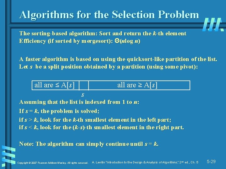
Algorithms for the Selection Problem The sorting-based algorithm: Sort and return the k-th element Efficiency (if sorted by mergesort): Θ(nlog n) A faster algorithm is based on using the quicksort-like partition of the list. Let s be a split position obtained by a partition (using some pivot): all are ≤ A[s] all are ≥ A[s] s Assuming that the list is indexed from 1 to n: If s = k, the problem is solved; if s > k, look for the k-th smallest element in the left part; if s < k, look for the (k-s)-th smallest element in the right part. Note: The algorithm can simply continue until s = k. Copyright © 2007 Pearson Addison-Wesley. All rights reserved. A. Levitin “Introduction to the Design & Analysis of Algorithms, ” 2 nd ed. , Ch. 5 5 -29

Tracing the Median / Selection Algorithm Here: n = 9, k = 9/2 = 5 Example: 4 1 10 9 7 12 8 2 15 array index 1 2 3 4 4 1 10 9 4 1 2 9 2 1 4 9 9 9 8 8 7 Solution: median is 8 Copyright © 2007 Pearson Addison-Wesley. All rights reserved. 5 6 7 7 7 7 8 12 12 8 9 8 8 2 8 10 12 10 9 15 15 15 --- s=3 < k=5 15 15 15 --- s=6 > k=5 --- s=k=5 A. Levitin “Introduction to the Design & Analysis of Algorithms, ” 2 nd ed. , Ch. 5 5 -30

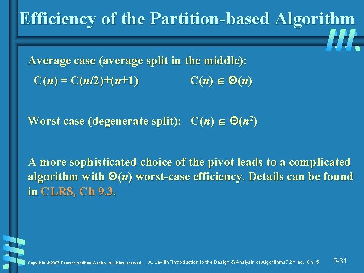
Efficiency of the Partition-based Algorithm Average case (average split in the middle): C(n) = C(n/2)+(n+1) C(n) Θ(n) Worst case (degenerate split): C(n) Θ(n 2) A more sophisticated choice of the pivot leads to a complicated algorithm with Θ(n) worst-case efficiency. Details can be found in CLRS, Ch 9. 3. Copyright © 2007 Pearson Addison-Wesley. All rights reserved. A. Levitin “Introduction to the Design & Analysis of Algorithms, ” 2 nd ed. , Ch. 5 5 -31

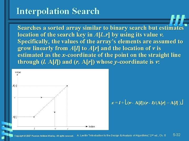
Interpolation Searches a sorted array similar to binary search but estimates location of the search key in A[l. . r] by using its value v. Specifically, the values of the array’s elements are assumed to grow linearly from A[l] to A[r] and the location of v is estimated as the x-coordinate of the point on the straight line through (l, A[l]) and (r, A[r]) whose y-coordinate is v: x = l + (v - A[l])(r - l)/(A[r] – A[l] ) Copyright © 2007 Pearson Addison-Wesley. All rights reserved. A. Levitin “Introduction to the Design & Analysis of Algorithms, ” 2 nd ed. , Ch. 5 5 -32

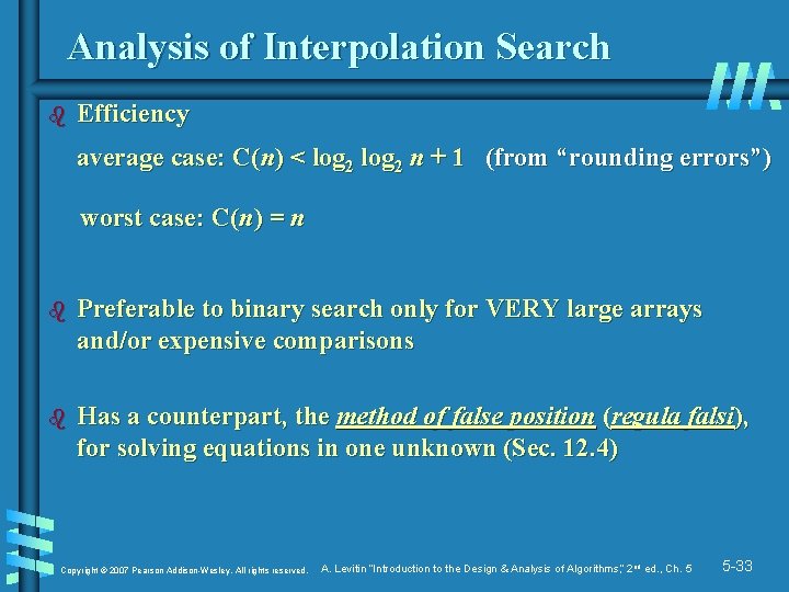
Analysis of Interpolation Search b Efficiency average case: C(n) < log 2 n + 1 (from “rounding errors”) worst case: C(n) = n b Preferable to binary search only for VERY large arrays and/or expensive comparisons b Has a counterpart, the method of false position (regula falsi), for solving equations in one unknown (Sec. 12. 4) Copyright © 2007 Pearson Addison-Wesley. All rights reserved. A. Levitin “Introduction to the Design & Analysis of Algorithms, ” 2 nd ed. , Ch. 5 5 -33

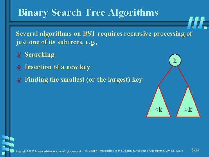
Binary Search Tree Algorithms Several algorithms on BST requires recursive processing of just one of its subtrees, e. g. , b Searching b Insertion of a new key b Finding the smallest (or the largest) key k <k Copyright © 2007 Pearson Addison-Wesley. All rights reserved. A. Levitin “Introduction to the Design & Analysis of Algorithms, ” 2 nd ed. , Ch. 5 >k 5 -34

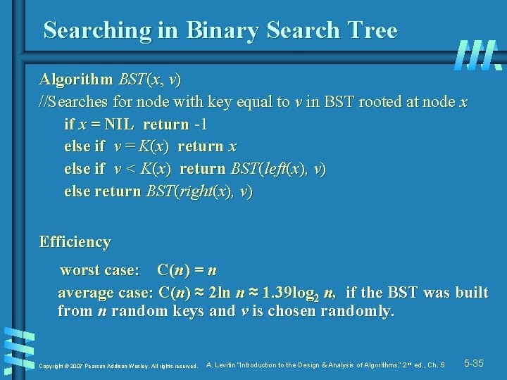
Searching in Binary Search Tree Algorithm BST(x, v) //Searches for node with key equal to v in BST rooted at node x if x = NIL return -1 else if v = K(x) return x else if v < K(x) return BST(left(x), v) else return BST(right(x), v) Efficiency worst case: C(n) = n average case: C(n) ≈ 2 ln n ≈ 1. 39 log 2 n, if the BST was built from n random keys and v is chosen randomly. Copyright © 2007 Pearson Addison-Wesley. All rights reserved. A. Levitin “Introduction to the Design & Analysis of Algorithms, ” 2 nd ed. , Ch. 5 5 -35

One-Pile Nim There is a pile of n chips. Two players take turn by removing from the pile at least 1 and at most m chips. (The number of chips taken can vary from move to move. ) The winner is the player that takes the last chip. Who wins the game – the player moving first or second, if both player make the best moves possible? It’s a good idea to analyze this and similar games “backwards”, i. e. , starting with n = 0, 1, 2, … Copyright © 2007 Pearson Addison-Wesley. All rights reserved. A. Levitin “Introduction to the Design & Analysis of Algorithms, ” 2 nd ed. , Ch. 5 5 -36

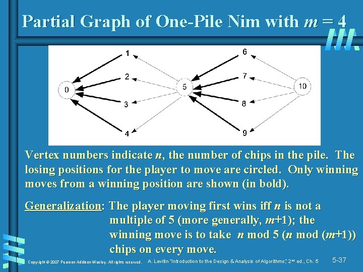
Partial Graph of One-Pile Nim with m = 4 Vertex numbers indicate n, the number of chips in the pile. The losing positions for the player to move are circled. Only winning moves from a winning position are shown (in bold). Generalization: The player moving first wins iff n is not a multiple of 5 (more generally, m+1); the winning move is to take n mod 5 (n mod (m+1)) chips on every move. Copyright © 2007 Pearson Addison-Wesley. All rights reserved. A. Levitin “Introduction to the Design & Analysis of Algorithms, ” 2 nd ed. , Ch. 5 5 -37