Chapter 5 Coding Learning Objectives LO 5 1

Chapter 5: Coding

Learning Objectives LO 5. 1 - Understand the basics of source encoding, its classifications and source-coding theorem. LO 5. 2 – Discuss source coding techniques including Shannon. Fano, Huffman, and Lempel-Ziv. LO 5. 3 – Implement error-control channel-coding techniques such as Hamming codes, cyclic codes, BCH code, Hadamard code, and LDPC code. LO 5. 4 – Illustrate the concept of convolution codes, Viterbi and

INTRODUCTION Figure 5. 0. 1 A Typical Transmission Model of Digital Data

5. 1 Basics of Source Encoding 5. 1. 1 Classification of Source Codes 5. 1. 2 Kraft-Mc. Millan Inequality 5. 1. 3 Source-Coding Theorem

Objectives and Need of Source Coding Source coding is the process by which data generated by a source is represented efficiently. The redundant data bits are reduced by applying the concepts of information theory. Objectives of source coding: - To form efficient descriptions of information for a given available data rate. - To allow data rates to obtain an acceptable efficient description of the source information. Need of source coding is for both analog sources and discrete sources.

Important Definitions Average Codeword Length: In physical terms, the average codeword length represents the average number of bits per source symbol used in the source encoding process. Code Efficiency: The ratio of minimum possible value of average codeword length to the average codeword length of the symbols used in the source encoding process. NOTE: The source encoder is said to be efficient when code efficiency approaches unity.

5. 1. 1 Classification of Source Codes Fixed-Length Source Codes Variable-Length Source Codes Distinct Codes Uniquely Decodable Codes Prefix Source Codes Instantaneous Source Codes Optimal Source Codes Entropy Coding

5. 1. 2 Kraft-Mc. Millan Inequality It specifies a condition on the codeword length of the prefix source code. ü If a code satisfies Kraft-Mc. Millan inequality condition, then it may or may not be a prefix code. ü If a code violates the Kraft-Mc. Millan inequality condition, then it is certain that it cannot be a prefix code.

5. 1. 3 Source Coding Theorem For a given discrete memoryless source, the average codeword length per symbol for any distortion-less source encoding scheme is bounded by the source entropy. The coding-efficiency of a source encoder is related to entropy and average codeword length as For M-ary source, the coding-efficiency is

5. 2 Source-Coding Techniques 5. 2. 1 Shannon-Fano Source Code 5. 2. 2 Huffman Source Code 5. 2. 3 Lempel-Ziv Code

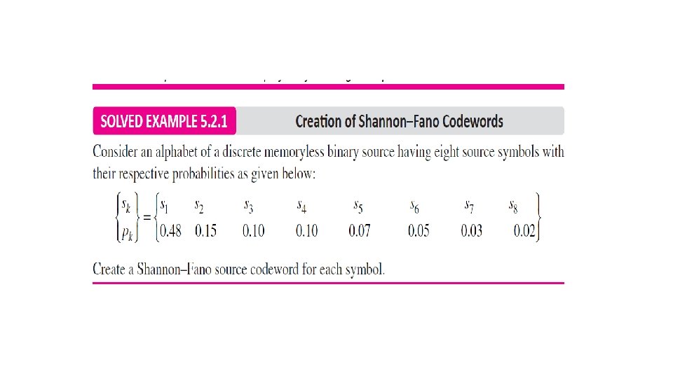
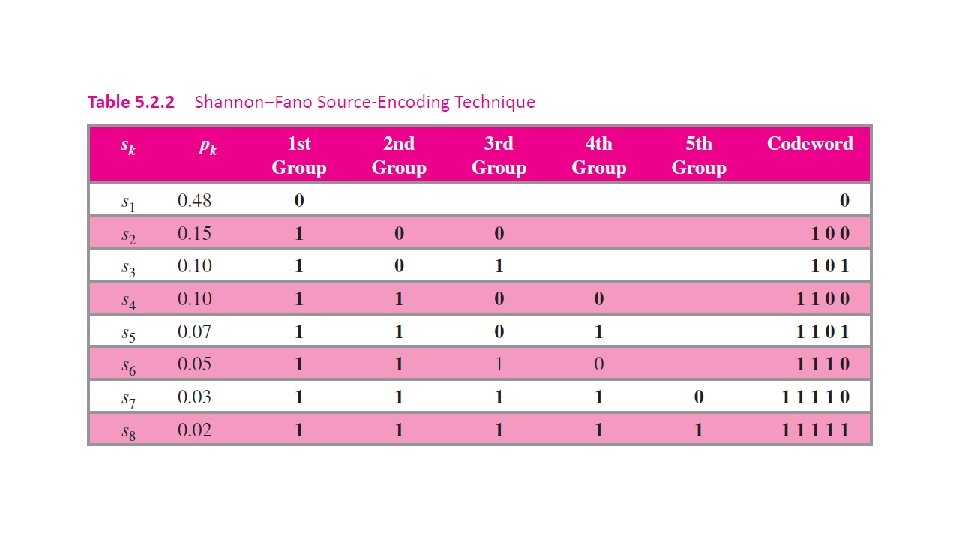
5. 2. 1 Shannon Fano Source Coding Step # Action to be Taken I Arrange the given source symbols in order of their specified decreasing probability. II Group them in two groups (for 2 -level encoder) or three groups (for 3 -level encoder) in such a way so that the sum of individual probability of source symbols in each group is nearly equal. III In case of 2 -level encoding, assign a binary digit 0 to source symbols contained in first group, and a binary digit 1 to source symbols contained in second group. In case of 3 -level encoding, assign a level -1 to source symbols contained in first group, a level 0 to source symbols contained in second group, and a level 1 to source symbols contained in third group. If any of the divided groups contains more than one symbol, divide them again in two or three groups, as the case may be, in such a way so that the sum of individual probability of source symbols in each group is nearly equal. The assignment of a binary level is done as described in step III above, Repeat the procedure specified in steps from IV and V any number of times until a final set of two or three groups containing one source symbol each is obtained. Assign a binary level to final two or three source symbols also as obtained in step V. IV V VI

5. 2. 2 Huffman Source Code Step # Action to be Taken I List the given source symbols in order of their specified decreasing probability. II IV V VI VII Assign a binary logic 0 and a binary logic 1 to the two source symbols of lowest probability in the list obtained in step I above. This is called splitting stage. Add the probability of these two source symbols and regard it as one new source symbol. This results into reduction of the size of the list of source symbols by one. Place the assigned probability of the new symbol high or low in the list with the rest of the symbols with their given probabilities. In case the assigned probability of the new symbol is equal to another probability in the reduced list, it may either may be placed higher (preferably) or lower than the original probability. It is presumed that whatever may be the placement (high or low), it is consistently adhered to throughout the encoding procedure. Repeat the procedure specified in steps from II to IV any number of times until a final set of two source symbols (one original and the other new) is obtained. Assign a binary logic 0 and a binary logic 1 to the final two source symbols also as obtained in step V above. This is known as Huffman Tree. Determine the codeword for each original source symbol by working backward and tracing the sequence of binary logic values 0 s and 1 s assigned to that symbol as well as its successors.

Example 5. 2. 7 Creation of Huffman Tree

5. 2. 3 Lampel-Ziv Code Lempel-Ziv code (LZ code) uses fixed-length codes to represent a variable number of source symbols. It does not require knowledge of a probabilistic model of the source. Step I: Parse the source data stream into segments that are the shortest strings not encountered previously Step II: Write the location of the prefix in binary followed by new last digit. If the parsing gives N number of strings for a given n-long sequence, then (rounded to the next integer) will be the number of binits required for describing prefix.

5. 3 Error-Control Channel Coding 5. 3. 1 Types of Errors and Error-Control Codes 5. 3. 2 Hamming Codes 5. 3. 3 Cyclic Codes 5. 3. 4 BCH Codes 5. 3. 5 Hadamard Codes 5. 3. 6 LDPC Codes

Essence of Channel Coding

5. 3. 1 Types of Errors and Error-Control Codes Random Errors Backward Error Correction (BEC) Burst Errors Forward Error Correction (BEC) Impulse Errors Single Bit Errors Linear Block Codes Multiple Bit Errors Convolution Codes Burst Errors Burst-Error Correction Codes

Linear Block Codes

Important Definitions Bit Error Rate (BER) – Theoretical expected value of the error performance which can be estimated mathematically. Error Detection – Process of monitoring data transmission and detecting when errors in data have occurred. Parity Bit – An additional bit to the bit pattern to make sure that the total number of 1’s is even or odd. Redundancy Checking – Adding extra bits to the data for the exclusive purpose of detecting transmission data errors. Code Rate – The ratio of number of information data bits (uncoded) and number of encoded data bits.

5. 3. 2 Hamming Codes Hamming code is the first class of (n, k) linear block code devised for error control. It is the form of non-systematic code in which the position of error control bits is arbitrary within a codeword. This expression is used to calculate the number of check bits, m. The Hamming code can be applied to data units of any length (k bits) using this relationship.

Example 5. 3. 3 Computation of Hamming Code

Example 5. 3. 4 Detection of Error with Hamming Code

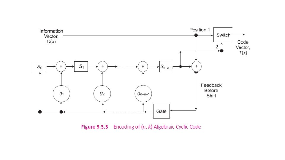
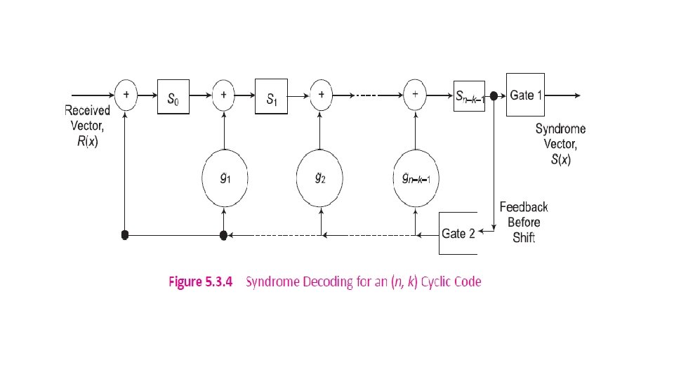
5. 3. 3 Cyclic Codes Cyclic code is a subclass of (n, k) linear block codes in which any cyclic shift of a codeword results in another valid codeword. Codes generated by a polynomial are called cyclic codes, and the resultant block codes are called cyclic redundancy check (CRC) codes.

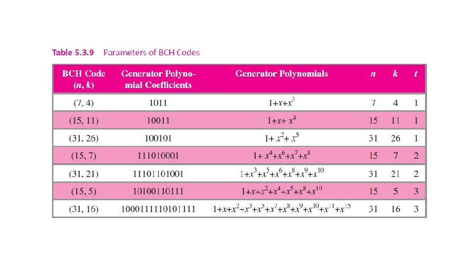
5. 3. 4 BCH Codes Named after its inventors, Bose-Chaudhuri-Hocquenghem, BCH code is one of the most important and powerful class of random-error-correcting cyclic polynomial codes over a finite field with a particular chosen generator polynomial.

5. 3. 5 Hadamard Codes

5. 3. 6 LDPC Codes Low-Density Parity Check (LDPC) Codes are a class of non-cyclic linear block codes. It is represented by a sparse parity-check matrix. • For regular LDPC codes, all rows as well as all columns have equal weights. • Irregular LDPC codes have a variable number of 1’s in the rows and in the columns.

Decoding Techniques for LDPC Codes Majority Logic (MLG) Decoding Bit-Flipping (BF) and Weighted Bit-Flipping (WBF) Decoding Algorithms Iterative Decoding based on Belief Propagation (IDBP) Algorithm A Posteriori Probability (APP) Decoding

5. 4 Convolution Coding and Decoding Convolution codes differ from block codes in that the encoder contains memory and the n encoder outputs at any given time unit depend not only on the k inputs at that time unit but also on m previous input blocks. The code rate is given as

Example 5. 4. 1 Generation of Convolution Code

Methods to describe a Convolution Code • State Diagram • Trellis Diagram • Tree Diagram or Code Tree

Example 5. 4. 6 State Diagram

A Trellis Diagram

Code Tree

Convolution Decoding

Figure 5. 4. 15 Trellis Diagram for Viterbi Decoding

5. 5 Burst Error-Correction Techniques 5. 5. 1 Interleaving 5. 5. 2 RS Codes 5. 5. 3 Turbo Codes

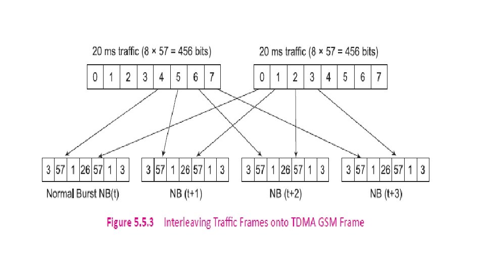
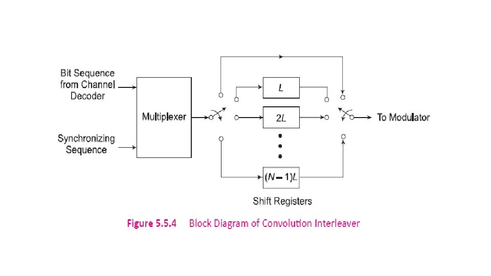
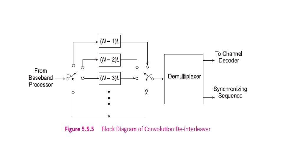
5. 5. 1 Interleaving is the process of dispersing the burst error into multiple individual errors which can then be detected and corrected by error control coding. Block Interleaver – A block of data symbols is written row by row as a n x m matrix and read column by column. Convolution Interleaver - It has memory, that is, its operation depends not only on current symbols but also on the previous symbols.

Types of Block Interleavers General Block Interleaver Odd-even Interleaver Algebraic Interleaver Helical Scan Interleaver Matrix Interleaver Random Interleaver

Figure 5. 5. 1 An Example of Block Interleaving

5. 5. 2 RS Codes

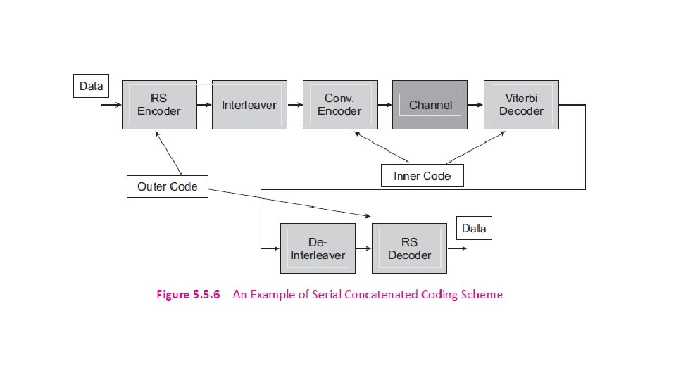
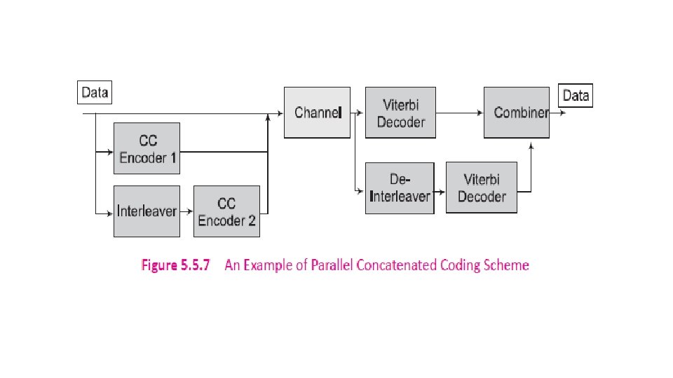
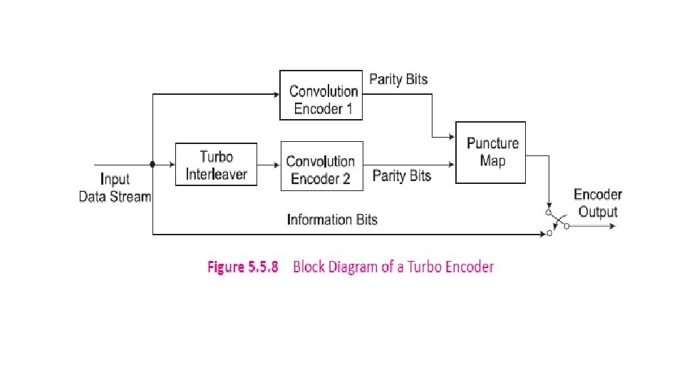
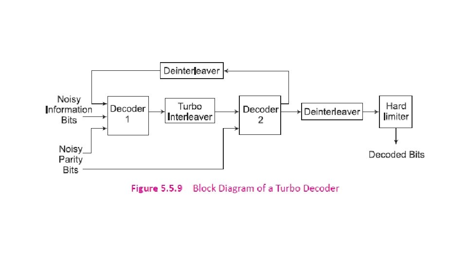
5. 5. 3 Turbo Codes Gallager (1961), Tanner (1981), and Berrou, Glavieux, and Thitimajshima invented Turbo codes in 1993. Turbo codes are based on concatenated coding. A concatenated code consists of two separated codes which are combined to form a larger code. A serial concatenation of codes is most often used for powerlimited systems such as transmitters on deep-space probes.

About the Author T. L. Singal graduated from National Institute of Technology, Kurukshetra and post-graduated from Punjab Technical university in Electronics & Communication Engineering. He began his career with Avionics Design Bureau, HAL, Hyderabad in 1981 and worked on Radar Communication Systems. Then he led R&D group in a Telecom company and successfully developed Multi-Access VHF Wireless Communication Systems. He visited Germany during 1990 -92. He executed international assignment as Senior Network Consultant with Flextronics Network Services, Texas, USA during 2000 -02. He was associated with Nokia, AT&T, Cingular Wireless and Nortel Networks, for optimization of 2 G/3 G Cellular Networks in USA. Since 2003, he is in teaching profession in reputed engineering colleges in India. He has number of technical research papers published in the IEEE Proceedings, Journals, and International/National Conferences. He has authored three text-books `Wireless Communications (2010)’, `Analog & Digital Communications (2012)’, and `Digital Communication (2015) with internationally renowned publisher Mc. Graw-Hill Education.

THANKS!