Chapter 5 Choice Budget set preference choice Optimal

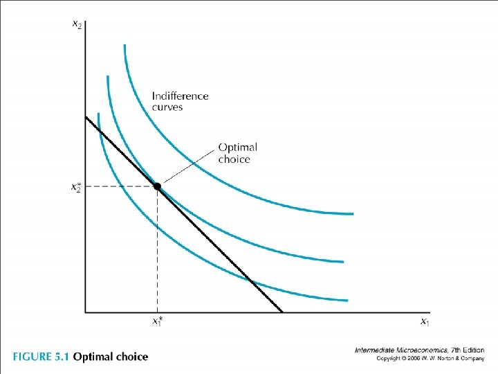
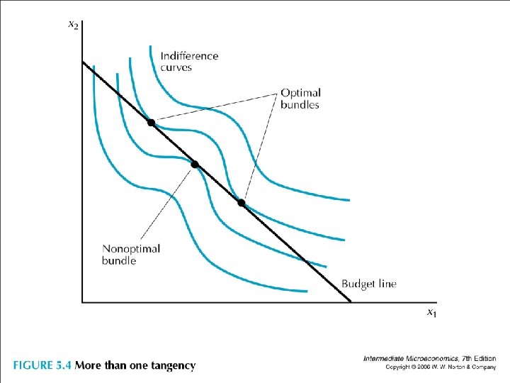
• Chapter 5 Choice • Budget set + preference → choice • Optimal choice: choose the best one can afford. Suppose the consumer chooses bundle A. A is optimal (A w B for any B in the budget set) ↔ the set of consumption bundles which is strictly preferred to A by this consumer cannot intersect with the budget set. (月亮形區 域)

• A optimal↔月亮形區域為空. • A optimal →月亮形區域為空? If not, then月亮形區域不為空, that means there exists a bundle B such that B s A and B is in the budget set. Then A is not optimal. • A optimal ←月亮形區域為空? All B such that B s A is not affordable, so for all B in the budget set, we must have A w B. Hence A is optimal.

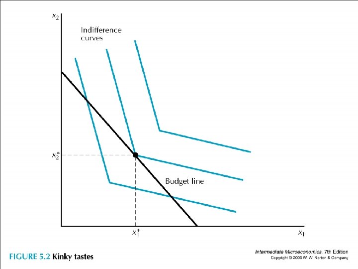
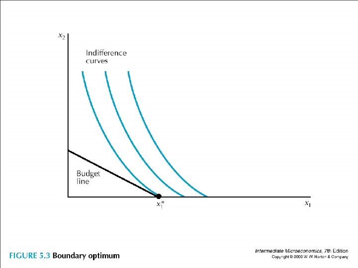
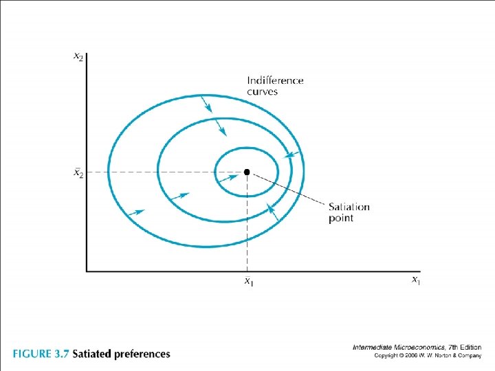
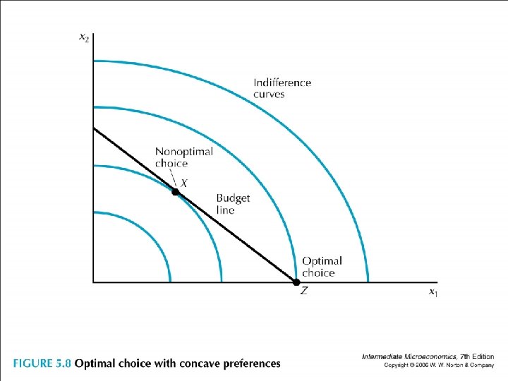
• The indifference curve tangent to the budget line is neither necessary nor sufficient for optimality. • Not necessary: kinked preferences (perfect complements), corner solution (vs. interior solution) (!!) (intuition) • Not sufficient: satiation or convexity is violated
, corner solution (vs. interior")
sufficient optimum necessary • Not necessary: kinked preferences (perfect complements), corner solution (vs. interior solution) (!!) (intuition) • Not sufficient: satiation or convexity is violated

• The usual tangent condition MRS 1, 2= -p 1/ p 2 has a nice interpretation. The MRS is the rate the consumer is willing to pay for an additional unit of good 1 in terms of good 2. The relative price ratio is the rate the market asks a consumer to pay for an additional unit of good 1 in terms of good 2. At optimum, these two rates are equal. (主觀相對價格 vs. 客觀相對價格)

• |MRS 1, 2| > p 1/ p 2, buy more of 1 • |MRS 1, 2| < p 1/ p 2, buy less of 1 • We now know what the optimal choice is, let us turn to demand since they are related. • The optimal choice of goods at some price and income is the consumer’s demanded bundle. A demand function gives you the optimal amount of each good as a function of prices and income faced by the consumer.
: the demand function • At")
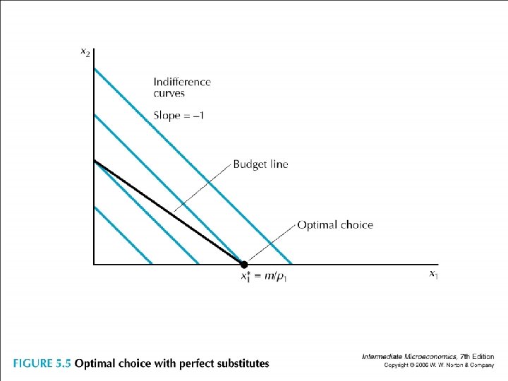
• x 1 (p 1, p 2, m): the demand function • At p 1, p 2, m, the consumer demands x 1 • Perfect substitutes: (graph) u(x 1, x 2) = x 1 + x 2 p 1 > p 2: x 1 = 0, x 2 = m/ p 2 p 1 = p 2: x 1 belongs to [0, m/ p 1] and x 2 = (m- p 1 x 1)/p 2 p 1 < p 2: x 1 = m/ p 1, x 2 = 0
 u(x 1, x 2) = min{x 1, x 2}")
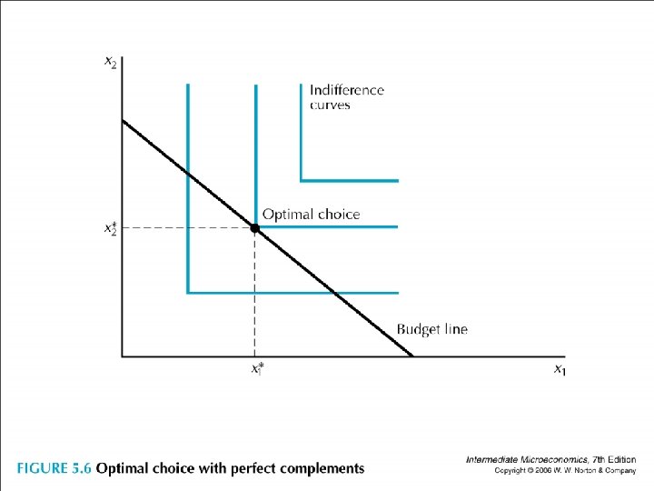
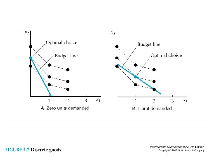
• Perfect complements: (graph) u(x 1, x 2) = min{x 1, x 2} x 1 = x 2 = m/ (p 1+ p 2) • Neutrals or bads: why spend money on them? • Discrete goods (just foolhardily compare) • Non convex preferences: corner solution
 = a lnx 1 + (1 -a)")
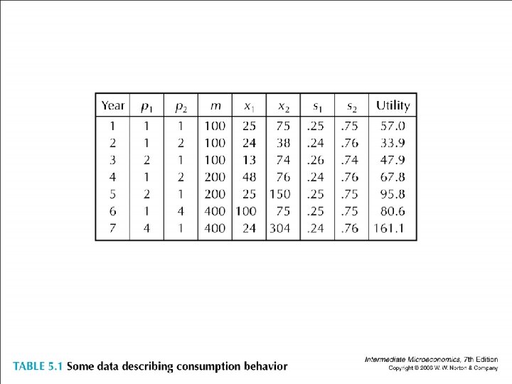
• Cobb-Douglas: u(x 1, x 2) = a lnx 1 + (1 -a) lnx 2 |MRS 1, 2| = p 1/ p 2, so (a/x 1)/[(1 -a)/x 2] = p 1/ p 2. This implies that a/(1 -a) = p 1 x 1/ p 2 x 2, so x 1 = am/ p 1 and x 2 = (1 -a)m/ p 2. This is useful if when we are estimating utility functions, we find that the expenditure share is fixed.

• Implication of the MRS condition: at equilibrium, we don’t need to know the preferences of each individual, we can infer that their MRS’ are the same. (This has an useful implication for Pareto efficiency as we will see later. )
 and milk (price: 1) • A")
• One small example: butter (price: 2) and milk (price: 1) • A new technology that will turn 3 units of milk into 1 unit of butter. Will this be profitable? • Another new tech that will turn 1 unit of butter into 3 units of milk. Will this be profitable?

• Choosing taxes: quantity tax and income tax • Suppose we impose a quantity tax of t dollars per unit of x 1. budget constraint: (p 1+t) x 1 + p 2 x 2 = m optimum: (x 1*, x 2*) so that (p 1+t) x 1* + p 2 x 2* = m income tax R* to raise the same revenue: R* = t x 1*

• optimum at income tax: p 1 x 1’+ p 2 x 2’ = m - R*, so (x 1*, x 2*) is affordable at the case of the income tax. hence, (x 1’, x 2’) w (x 1*, x 2*). (graph)
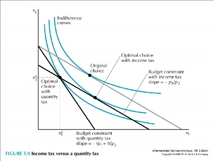

• Income tax better than quantity tax? two caveats: one consumer, uniform income tax vs. uniform quantity tax (think about the person who does not consume good 1) tax avoidance or income tax discourages earning ignore supply side
- Slides: 25