Chapter 5 A Closed Economy OnePeriod Macroeconomic Model



- Slides: 46

Chapter 5 A Closed. Economy One-Period Macroeconomic Model Copyright © 2014 Pearson Education, Inc.

Chapter 5 Topics • Introduce the government. • Construct closed-economy one-period macroeconomic model, which has: (i) representative consumer; (ii) representative firm; (iii) government. • Economic efficiency and Pareto optimality. • Experiments: Increases in government spending and total factor productivity. • Consider a distorting tax on wage income and study the Laffer curve. • Public goods: How large should the government be? © 2014 Pearson Education, Inc. 1 -2

Closed-Economy One-Period Macro Model • • Representative Consumer Representative Firm Competitive Equilibrium Experiments: What does the model tell us are the effects of changes in government spending and in total factor productivity? © 2014 Pearson Education, Inc. 1 -3

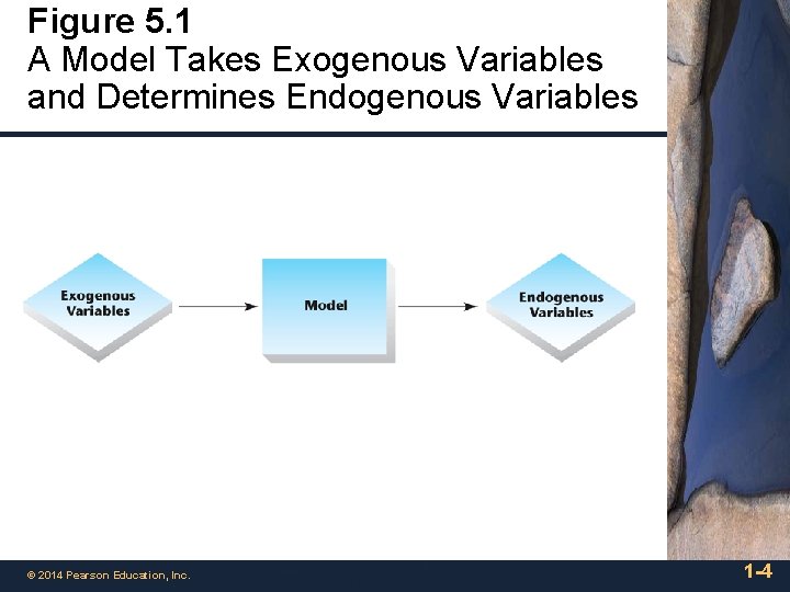
Figure 5. 1 A Model Takes Exogenous Variables and Determines Endogenous Variables © 2014 Pearson Education, Inc. 1 -4

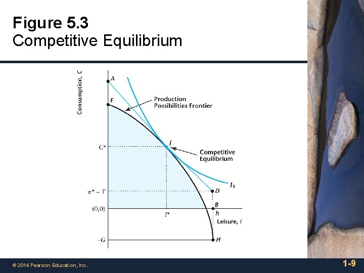
Competitive Equilibrium • • Representative consumer optimizes given market prices. Representative firm optimizes given market prices. The labor market clears. The government budget constraint is satisfied, or G = T. © 2014 Pearson Education, Inc. 1 -5

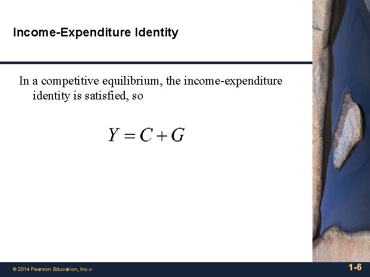
Income-Expenditure Identity In a competitive equilibrium, the income-expenditure identity is satisfied, so © 2014 Pearson Education, Inc. v 1 -6

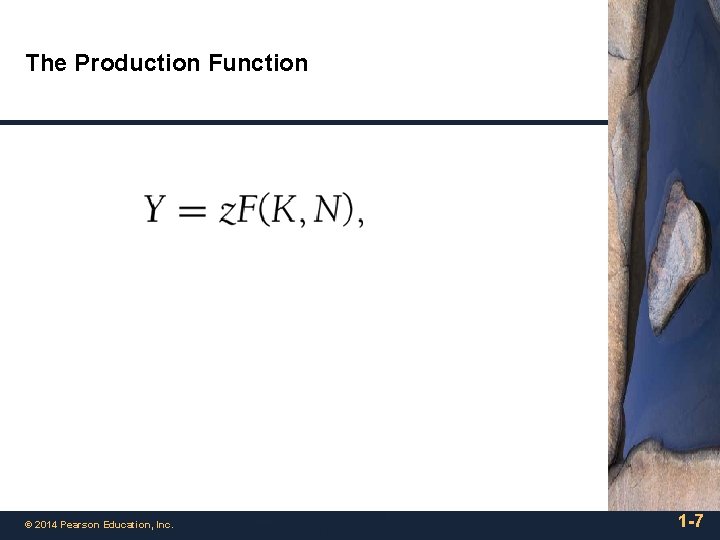
The Production Function © 2014 Pearson Education, Inc. 1 -7

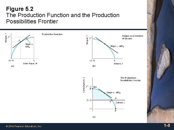
Figure 5. 2 The Production Function and the Production Possibilities Frontier © 2014 Pearson Education, Inc. 1 -8

Figure 5. 3 Competitive Equilibrium © 2014 Pearson Education, Inc. 1 -9

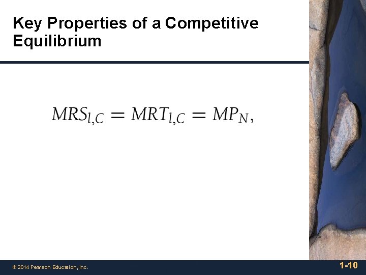
Key Properties of a Competitive Equilibrium © 2014 Pearson Education, Inc. 1 -10

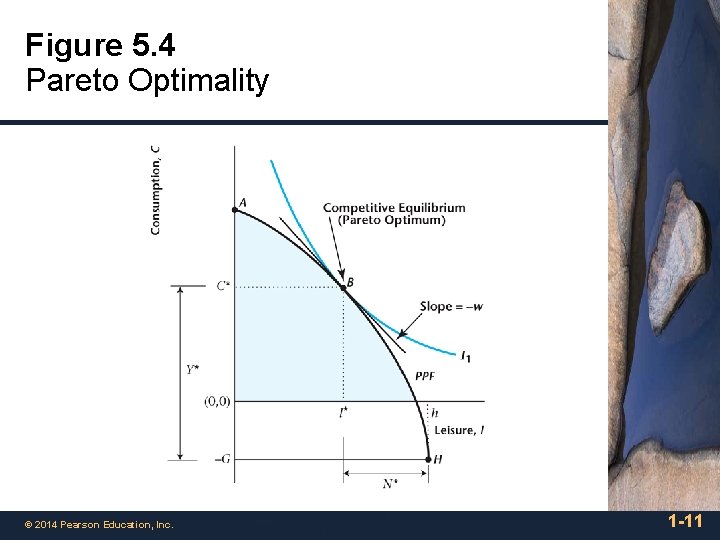
Figure 5. 4 Pareto Optimality © 2014 Pearson Education, Inc. 1 -11

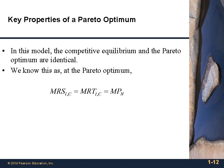
Key Properties of a Pareto Optimum • In this model, the competitive equilibrium and the Pareto optimum are identical. • We know this as, at the Pareto optimum, © 2014 Pearson Education, Inc. 1 -12

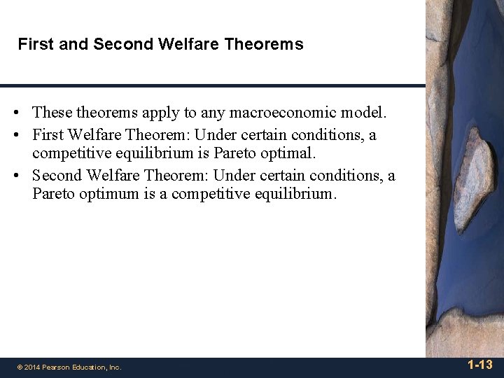
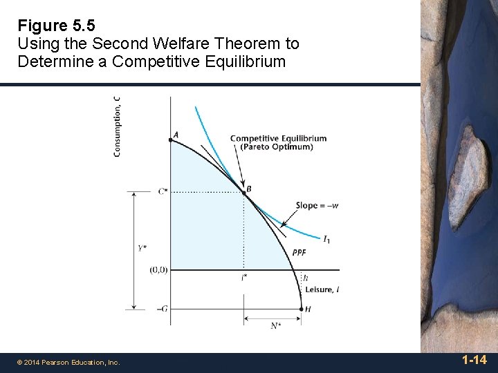
First and Second Welfare Theorems • These theorems apply to any macroeconomic model. • First Welfare Theorem: Under certain conditions, a competitive equilibrium is Pareto optimal. • Second Welfare Theorem: Under certain conditions, a Pareto optimum is a competitive equilibrium. © 2014 Pearson Education, Inc. 1 -13

Figure 5. 5 Using the Second Welfare Theorem to Determine a Competitive Equilibrium © 2014 Pearson Education, Inc. 1 -14

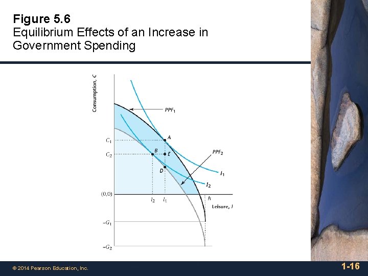
Effects of an Increase in G • Essentially a pure income effect • C decreases, l decreases, Y increases, w falls © 2014 Pearson Education, Inc. 1 -15

Figure 5. 6 Equilibrium Effects of an Increase in Government Spending © 2014 Pearson Education, Inc. 1 -16

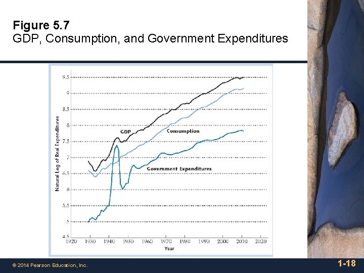
World War II Increase in G • Very large increase in G. • Y increases, C decreases by a small amount. © 2014 Pearson Education, Inc. 1 -17

Figure 5. 7 GDP, Consumption, and Government Expenditures © 2014 Pearson Education, Inc. 1 -18

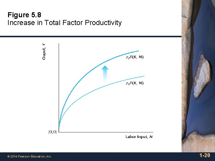
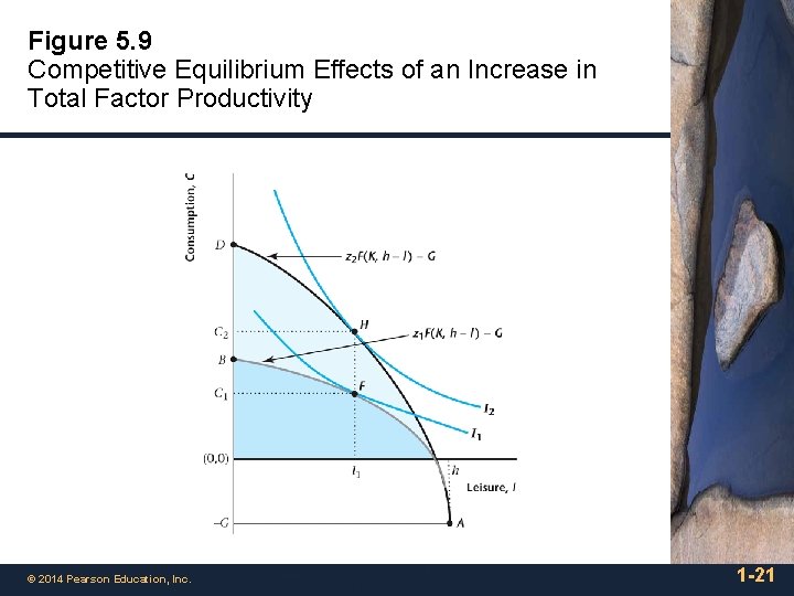
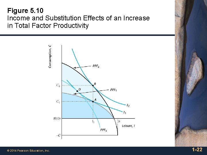
Effects of an Increase in z (or an increase in K) • PPF shifts out, and becomes steeper – income and substitution effects are involved. • C increases, l may increase or decrease, Y increases, w increases. © 2014 Pearson Education, Inc. 1 -19

Figure 5. 8 Increase in Total Factor Productivity © 2014 Pearson Education, Inc. 1 -20

Figure 5. 9 Competitive Equilibrium Effects of an Increase in Total Factor Productivity © 2014 Pearson Education, Inc. 1 -21

Figure 5. 10 Income and Substitution Effects of an Increase in Total Factor Productivity © 2014 Pearson Education, Inc. 1 -22

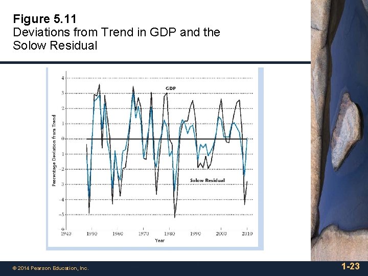
Figure 5. 11 Deviations from Trend in GDP and the Solow Residual © 2014 Pearson Education, Inc. 1 -23

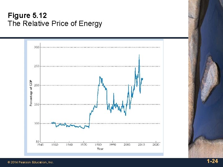
Figure 5. 12 The Relative Price of Energy © 2014 Pearson Education, Inc. 1 -24

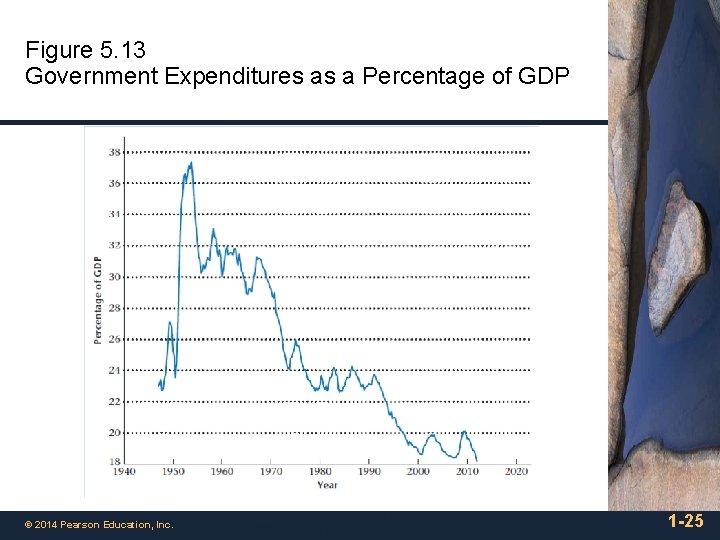
Figure 5. 13 Government Expenditures as a Percentage of GDP © 2014 Pearson Education, Inc. 1 -25

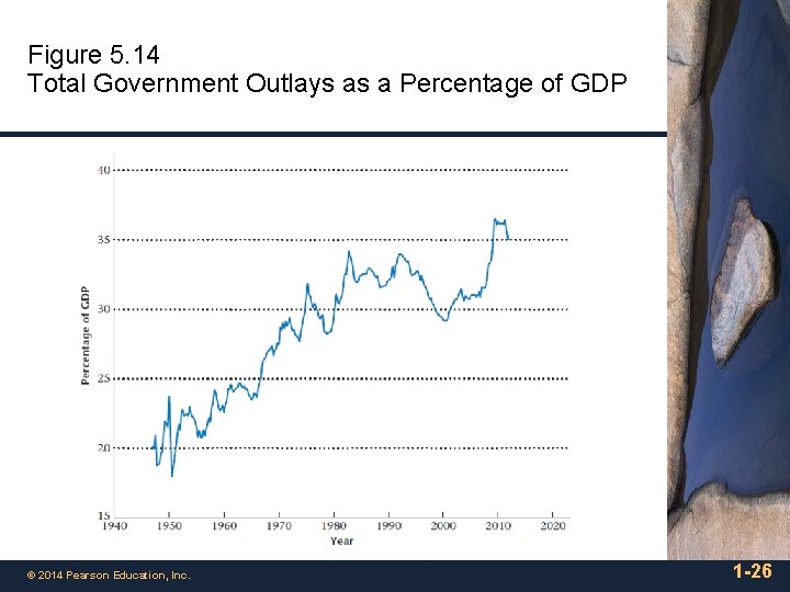
Figure 5. 14 Total Government Outlays as a Percentage of GDP © 2014 Pearson Education, Inc. 1 -26

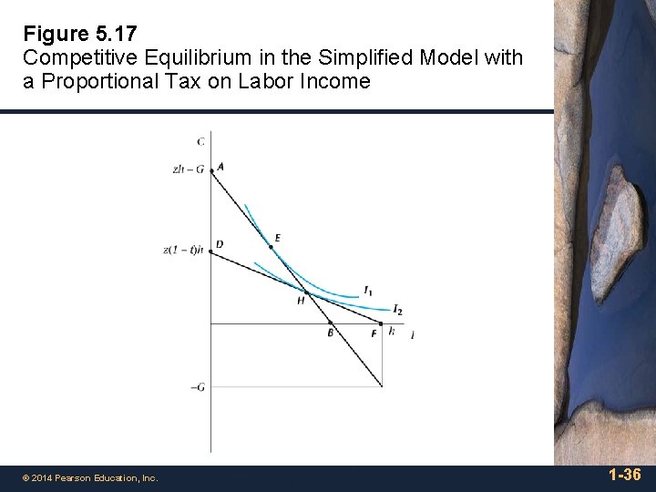
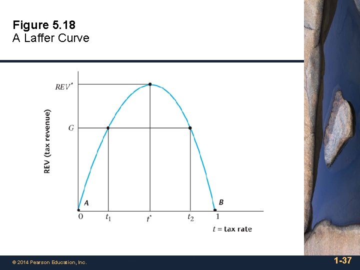
A Simplifed Model with a Proportional Income Tax • Use the model to study the incentive effects of the income tax, and to derive the “Laffer curve. ” © 2014 Pearson Education, Inc. 1 -27

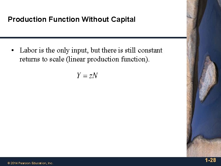
Production Function Without Capital • Labor is the only input, but there is still constant returns to scale (linear production function). © 2014 Pearson Education, Inc. 1 -28

Production Possibilities Frontier © 2014 Pearson Education, Inc. 1 -29

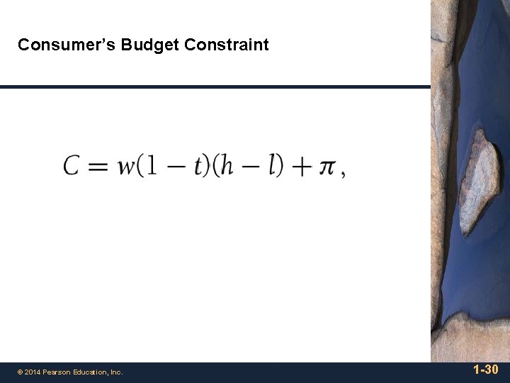
Consumer’s Budget Constraint © 2014 Pearson Education, Inc. 1 -30

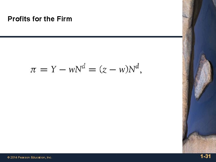
Profits for the Firm © 2014 Pearson Education, Inc. 1 -31

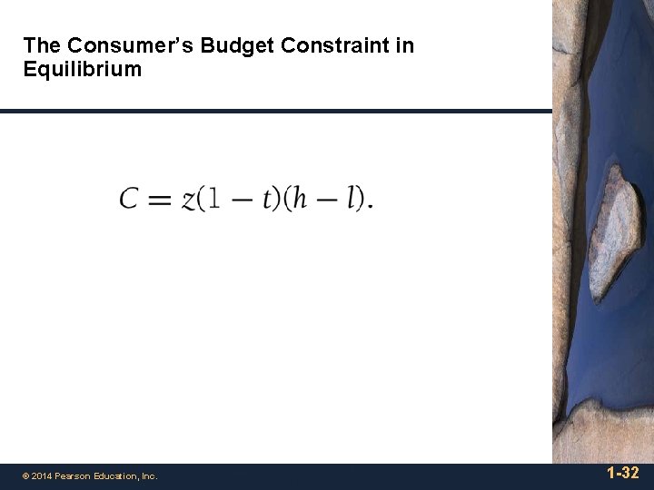
The Consumer’s Budget Constraint in Equilibrium © 2014 Pearson Education, Inc. 1 -32

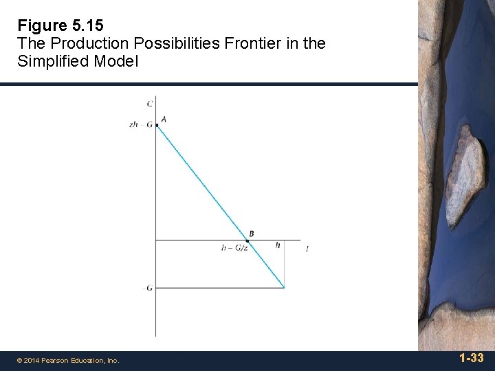
Figure 5. 15 The Production Possibilities Frontier in the Simplified Model © 2014 Pearson Education, Inc. 1 -33

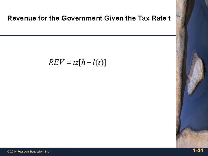
Revenue for the Government Given the Tax Rate t © 2014 Pearson Education, Inc. 1 -34

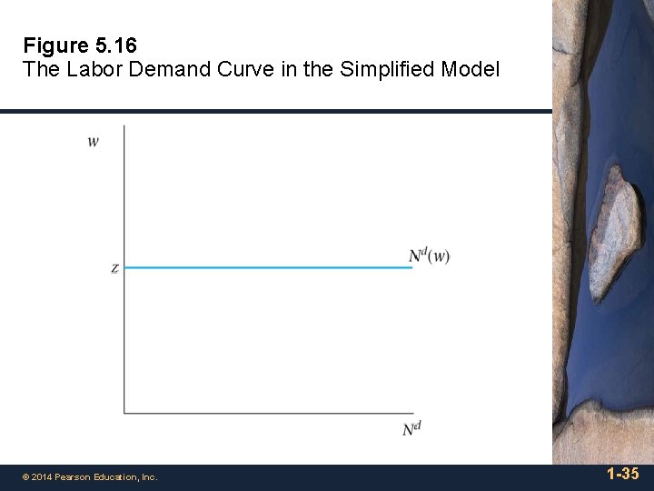
Figure 5. 16 The Labor Demand Curve in the Simplified Model © 2014 Pearson Education, Inc. 1 -35

Figure 5. 17 Competitive Equilibrium in the Simplified Model with a Proportional Tax on Labor Income © 2014 Pearson Education, Inc. 1 -36

Figure 5. 18 A Laffer Curve © 2014 Pearson Education, Inc. 1 -37

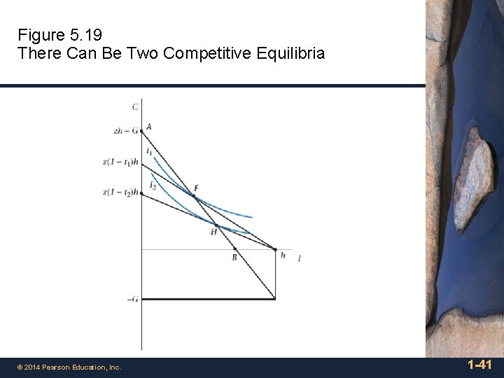
A Model of Public Goods: How Large Should the Government Be? • To this point, we have assumed that government spending is to acquire goods that are thrown away. • Economically, defense spending works like this – defense may make us better off, but it diverts resources from other uses. • What if we allow for public goods – e. g. parks, public transportation, health services – that provide direct benefits to the private sector. © 2014 Pearson Education, Inc. 1 -38

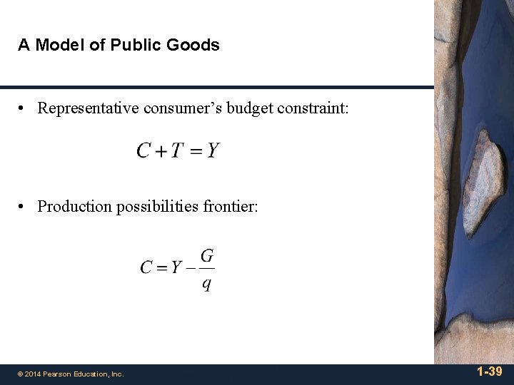
A Model of Public Goods • Representative consumer’s budget constraint: • Production possibilities frontier: © 2014 Pearson Education, Inc. 1 -39

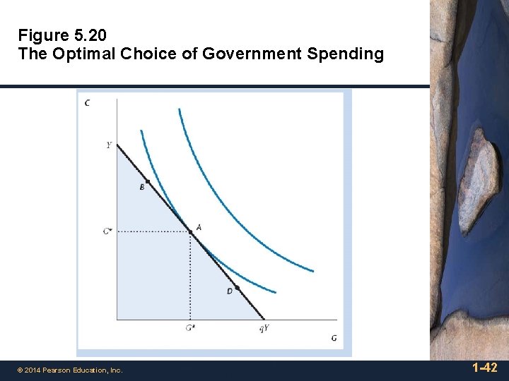
The Optimal Choice of Government Spending • The government chooses G to make the representative consumer as well off as possible. • G chosen so that the marginal rate of substitution of private for public goods equals the marginal rate of transformation. © 2014 Pearson Education, Inc. 1 -40

Figure 5. 19 There Can Be Two Competitive Equilibria © 2014 Pearson Education, Inc. 1 -41

Figure 5. 20 The Optimal Choice of Government Spending © 2014 Pearson Education, Inc. 1 -42

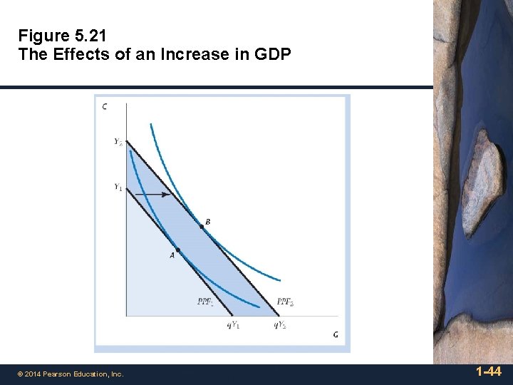
What Happens to the Optimal Choice of G when Y increases? • This works like a pure income effect. • Private consumption and government spending both increase. • Wealthier countries choose to have larger governments – but not clear whether G/Y increases or decreases. Is G a luxury good or an inferior good? © 2014 Pearson Education, Inc. 1 -43

Figure 5. 21 The Effects of an Increase in GDP © 2014 Pearson Education, Inc. 1 -44

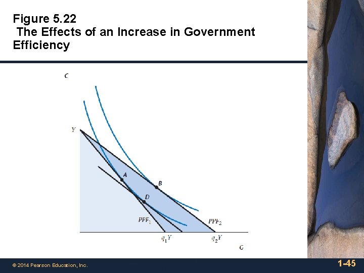
Figure 5. 22 The Effects of an Increase in Government Efficiency © 2014 Pearson Education, Inc. 1 -45

What Happens if the Government Becomes More Efficient? • q increases – can produce more G for a given input of private goods. • Income and substitution effects. • G increases, but private consumption may increase or decrease. © 2014 Pearson Education, Inc. 1 -46