CHAPTER 4 Working and Understanding Matrices in MATLAB

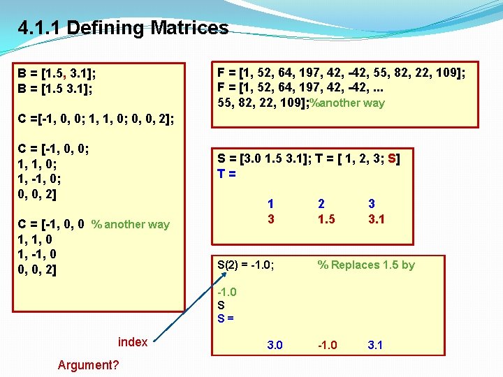
4. 1. 1 Defining Matrices F = [1, 52, 64, 197, 42, -42, 55, 82, 22, 109]; F = [1, 52, 64, 197, 42, -42, . . . 55, 82, 22, 109]; %another way B = [1. 5, 3. 1]; B = [1. 5 3. 1]; C =[-1, 0, 0; 1, 1, 0; 0, 0, 2]; C = [-1, 0, 0; 1, 1, 0; 1, -1, 0; 0, 0, 2] S = [3. 0 1. 5 3. 1]; T = [ 1, 2, 3; S] T= C = [-1, 0, 0 % another way 1, 1, 0 1, -1, 0 0, 0, 2] 1 3 S(2) = -1. 0; 2 1. 5 3 3. 1 % Replaces 1. 5 by -1. 0 S S= index Argument? 3. 0 -1. 0 3. 1

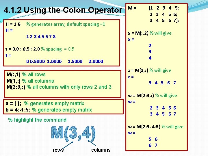
4. 1. 2 Using the Colon Operator H = 1: 8 H= % generates array, default spacing =1 12345678 t = 0. 0 : 0. 5 : 2. 0 % spacing = 0. 5 t= 0 0. 5000 1. 0000 1. 5000 2. 0000 M(: , 1) % all rows M(1, : ) % all columns M(2: 3, : ) % all columns with only rows 2 and 3 a = [ ]; % generates empty matrix b = 4: -1: 5; % generates empty matrix % highlight the command M(3, 4) rows columns M= [1 2 3 4 5; 2 3 4 5 6; 3 4 5 6 7]; x = M(: , 2) % will give x= 2 3 4 z = M(3, : ) % will give z= 3 4 5 6 7 w = M(2: 3, : ) % will give w= 2 3 4 5 6 7 w = M(2: 3, 4: 5) % will give w= 5 6 6 7

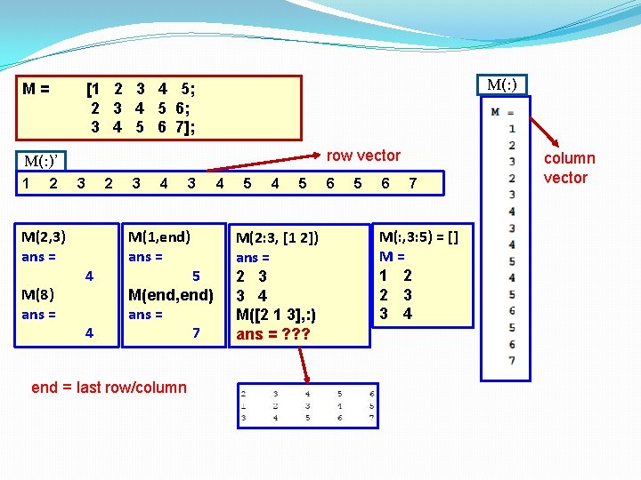
M= M(: ) [1 2 3 4 5; 2 3 4 5 6; 3 4 5 6 7]; row vector M(: )’ 1 2 M(2, 3) ans = M(8) ans = 3 4 4 2 3 4 3 M(1, end) ans = 5 M(end, end) ans = 7 end = last row/column 4 5 M(2: 3, [1 2]) ans = 2 3 3 4 M([2 1 3], : ) ans = ? ? ? 6 5 6 7 M(: , 3: 5) = [] M= 1 2 2 3 3 4 column vector

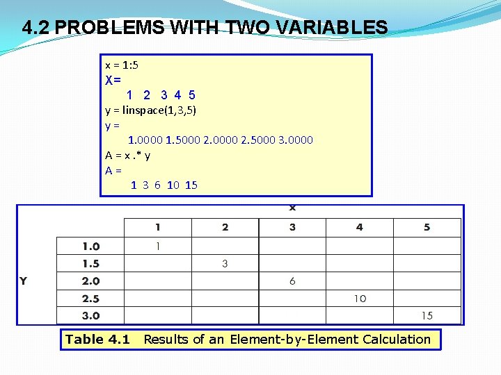
4. 2 PROBLEMS WITH TWO VARIABLES x = 1: 5 X= 1 2 3 4 5 y = linspace(1, 3, 5) y= 1. 0000 1. 5000 2. 0000 2. 5000 3. 0000 A = x. * y A= 1 3 6 10 15 Table 4. 1 Results of an Element-by-Element Calculation

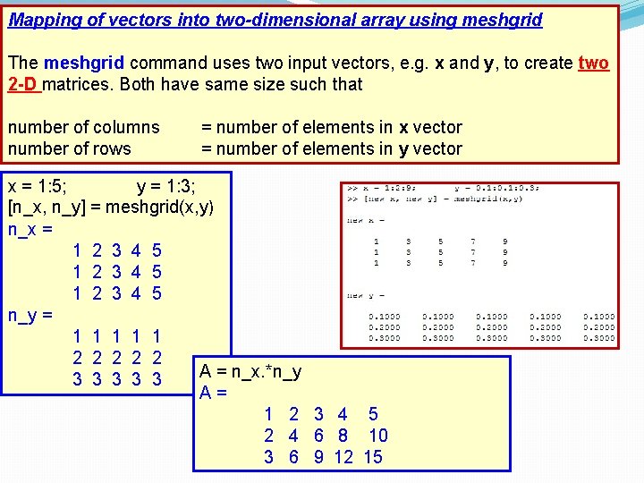
Mapping of vectors into two-dimensional array using meshgrid The meshgrid command uses two input vectors, e. g. x and y, to create two 2 -D matrices. Both have same size such that number of columns number of rows = number of elements in x vector = number of elements in y vector x = 1: 5; y = 1: 3; [n_x, n_y] = meshgrid(x, y) n_x = 1 2 3 4 5 n_y = 1 1 1 2 2 2 A = n_x. *n_y 3 3 3 A = 1 2 3 4 5 2 4 6 8 10 3 6 9 12 15

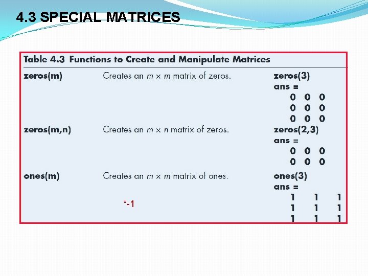
4. 3 SPECIAL MATRICES *-1

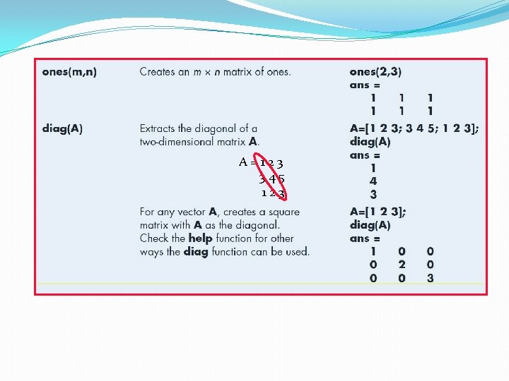
A = 1 2 3 3 4 5 1 2 3

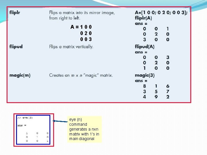
A=100 020 003 eye (n) command generates a nxn matrix with 1’s in main diagonal

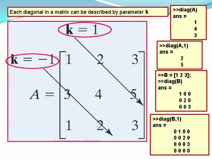
Each diagonal in a matrix can be described by parameter k >>diag(A) ans = 1 4 3 >>diag(A, 1) ans = 2 5 >>B = [1 2 3]; >>diag(B) ans = 100 020 003 >>diag(B, 1) ans = 0100 0020 0003 0000

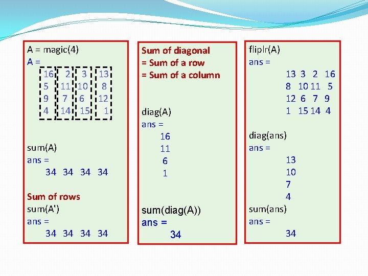
A = magic(4) A= 16 2 3 13 5 11 10 8 9 7 6 12 4 14 15 1 Sum of diagonal = Sum of a row = Sum of a column sum(A) ans = 34 34 diag(A) ans = 16 11 6 1 Sum of rows sum(A') ans = 34 34 sum(diag(A)) ans = 34 fliplr(A) ans = 13 3 2 8 10 11 12 6 7 1 15 14 diag(ans) ans = 13 10 7 4 sum(ans) ans = 34 16 5 9 4

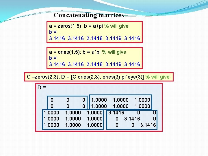
Concatenating matrices a = zeros(1, 5); b = a+pi % will give b = 3. 1416 a = ones(1, 5); b = a*pi % will give b = 3. 1416 C =zeros(2, 3); D = [C ones(2, 3); ones(3) pi*eye(3)] % will give D = 0 0 0 1. 0000 1. 0000 3. 1416 0 1. 0000 0 3. 1416

Ex. 4. 1

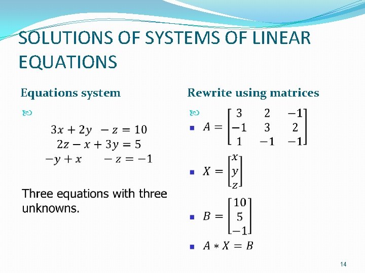
SOLUTIONS OF SYSTEMS OF LINEAR EQUATIONS Equations system Rewrite using matrices 14

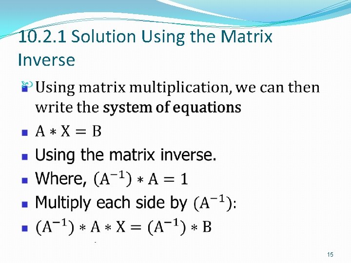
10. 2. 1 Solution Using the Matrix Inverse 15

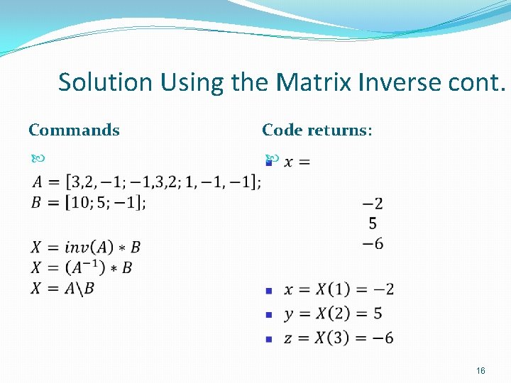
Solution Using the Matrix Inverse cont. Commands Code returns: 16

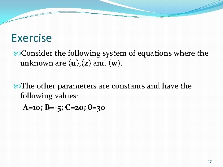
Exercise Consider the following system of equations where the unknown are (u), (z) and (w). The other parameters are constants and have the following values: A=10; B=-5; C=20; θ=30 17

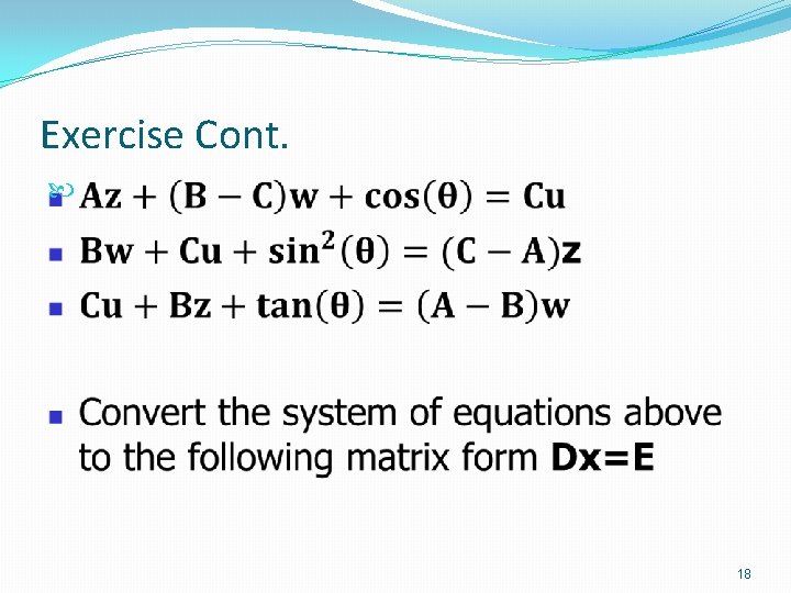
Exercise Cont. 18

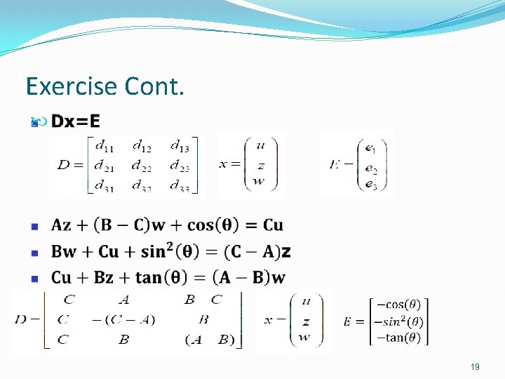
Exercise Cont. 19

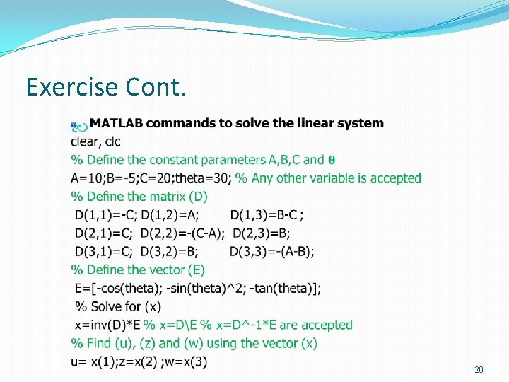
Exercise Cont. 20