Chapter 4 TwoLevel Systems Twolevel systems 4 C

Chapter 4 Two-Level Systems

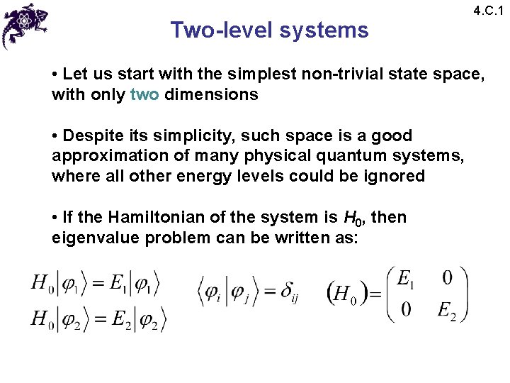
Two-level systems 4. C. 1 • Let us start with the simplest non-trivial state space, with only two dimensions • Despite its simplicity, such space is a good approximation of many physical quantum systems, where all other energy levels could be ignored • If the Hamiltonian of the system is H 0, then eigenvalue problem can be written as:

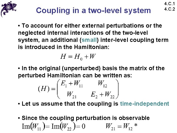
Coupling in a two-level system 4. C. 1 4. C. 2 • To account for either external perturbations or the neglected internal interactions of the two-level system, an additional (small) inter-level coupling term is introduced in the Hamiltonian: • In the original (unperturbed) basis the matrix of the perturbed Hamiltonian can be written as: • Let us assume that the coupling is time-independent • Since the coupling perturbation is observable

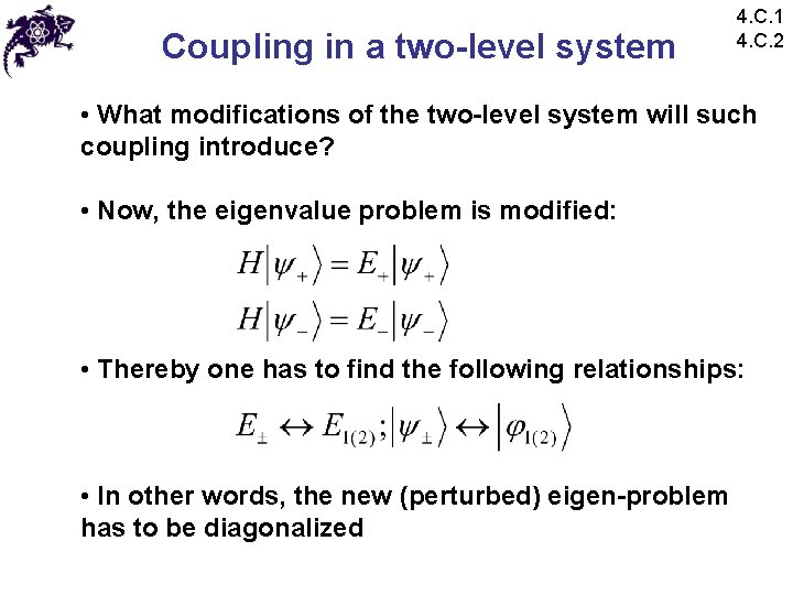
Coupling in a two-level system 4. C. 1 4. C. 2 • What modifications of the two-level system will such coupling introduce? • Now, the eigenvalue problem is modified: • Thereby one has to find the following relationships: • In other words, the new (perturbed) eigen-problem has to be diagonalized

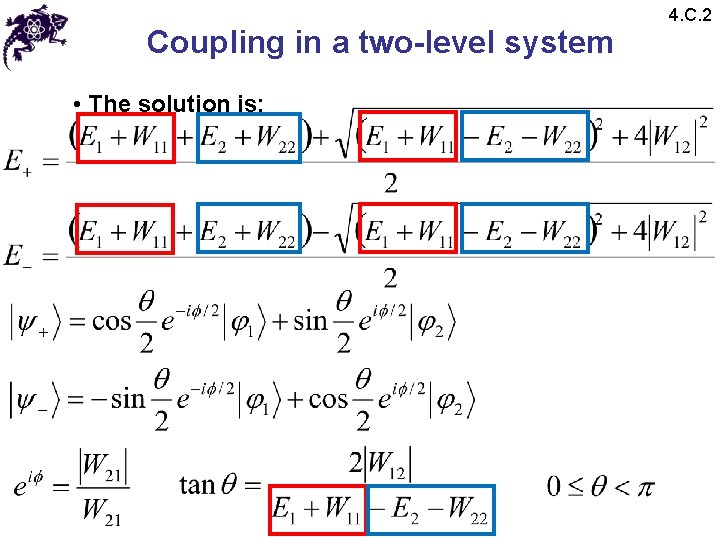
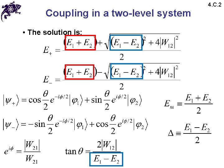
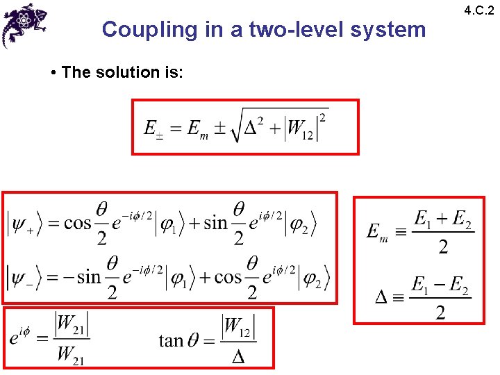
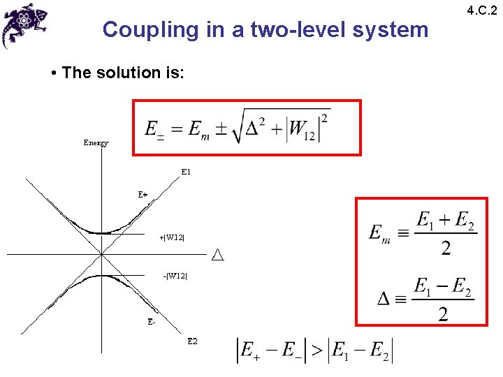
Coupling in a two-level system • The solution is: 4. C. 2

Coupling in a two-level system • The solution is: 4. C. 2

Coupling in a two-level system • The solution is: 4. C. 2

Coupling in a two-level system • The solution is: 4. C. 2

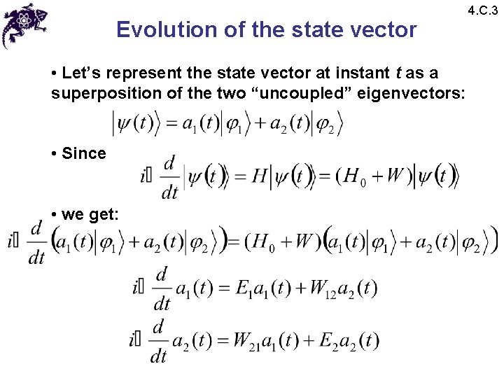
Evolution of the state vector • Let’s represent the state vector at instant t as a superposition of the two “uncoupled” eigenvectors: • Since • we get: 4. C. 3

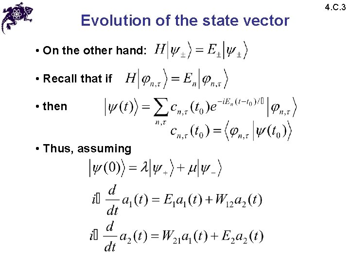
Evolution of the state vector • On the other hand: • Recall that if • then • Thus, assuming 4. C. 3

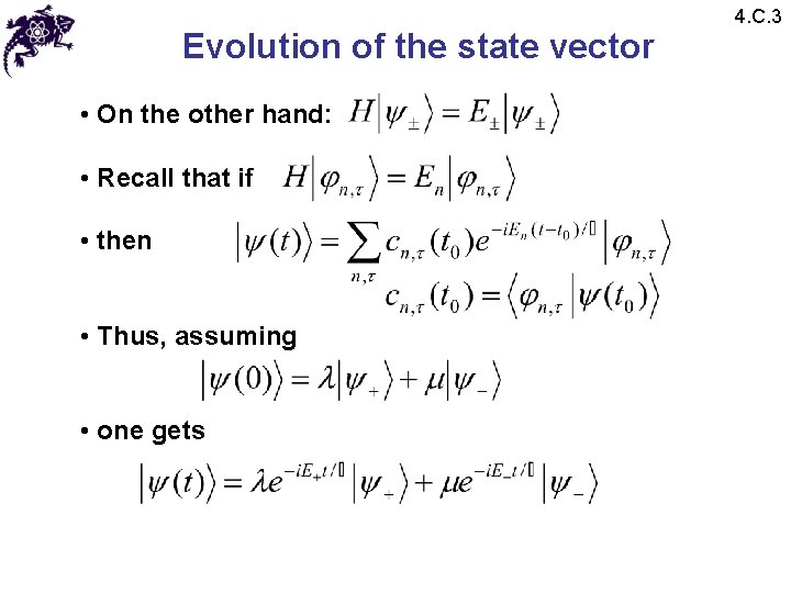
Evolution of the state vector • On the other hand: • Recall that if • then • Thus, assuming • one gets 4. C. 3

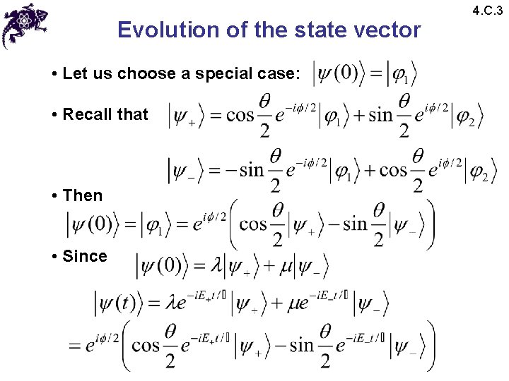
Evolution of the state vector • Let us choose a special case: • Recall that • Then • Since 4. C. 3

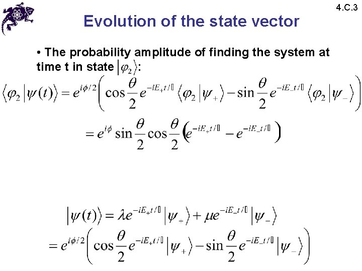
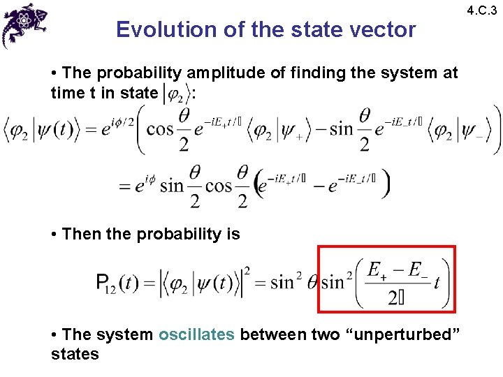
Evolution of the state vector • The probability amplitude of finding the system at time t in state : 4. C. 3

Evolution of the state vector • The probability amplitude of finding the system at time t in state : • Then the probability is • The system oscillates between two “unperturbed” states 4. C. 3

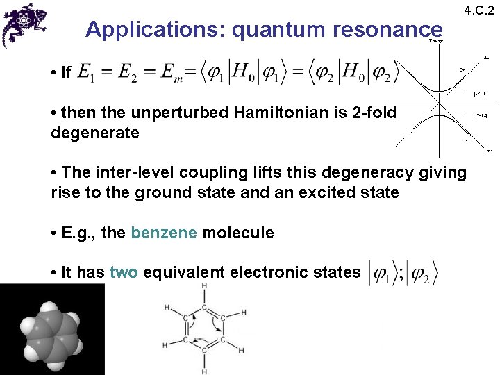
Applications: quantum resonance 4. C. 2 • If • then the unperturbed Hamiltonian is 2 -fold degenerate • The inter-level coupling lifts this degeneracy giving rise to the ground state and an excited state • E. g. , the benzene molecule • It has two equivalent electronic states

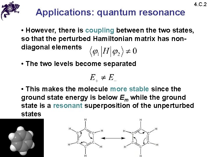
Applications: quantum resonance 4. C. 2 • However, there is coupling between the two states, so that the perturbed Hamiltonian matrix has nondiagonal elements • The two levels become separated • This makes the molecule more stable since the ground state energy is below Em while the ground state is a resonant superposition of the unperturbed states

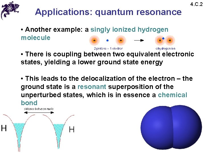
Applications: quantum resonance 4. C. 2 • Another example: a singly ionized hydrogen molecule • There is coupling between two equivalent electronic states, yielding a lower ground state energy • This leads to the delocalization of the electron – the ground state is a resonant superposition of the unperturbed states, which is in essence a chemical bond

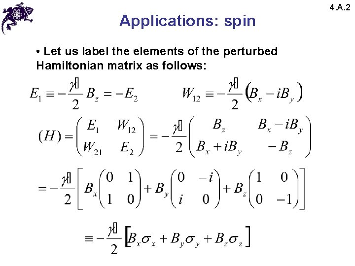
Applications: spin • Let us label the elements of the perturbed Hamiltonian matrix as follows: 4. A. 2

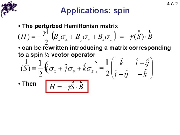
Applications: spin 4. A. 2 • The perturbed Hamiltonian matrix • can be rewritten introducing a matrix corresponding to a spin ½ vector operator • Then

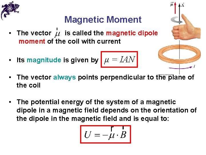
Magnetic Moment • The vector is called the magnetic dipole moment of the coil with current • Its magnitude is given by μ = IAN • The vector always points perpendicular to the plane of the coil • The potential energy of the system of a magnetic dipole in a magnetic field depends on the orientation of the dipole in the magnetic field and is equal to:

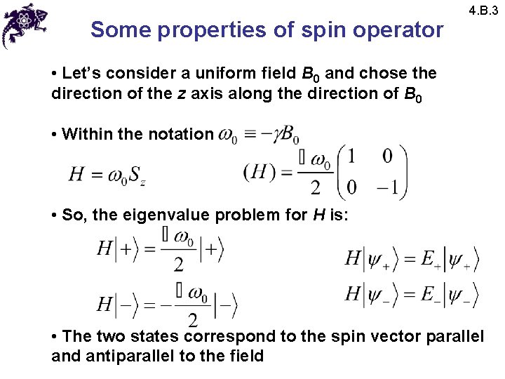
Some properties of spin operator 4. B. 3 • Let’s consider a uniform field B 0 and chose the direction of the z axis along the direction of B 0 • Within the notation • So, the eigenvalue problem for H is: • The two states correspond to the spin vector parallel and antiparallel to the field

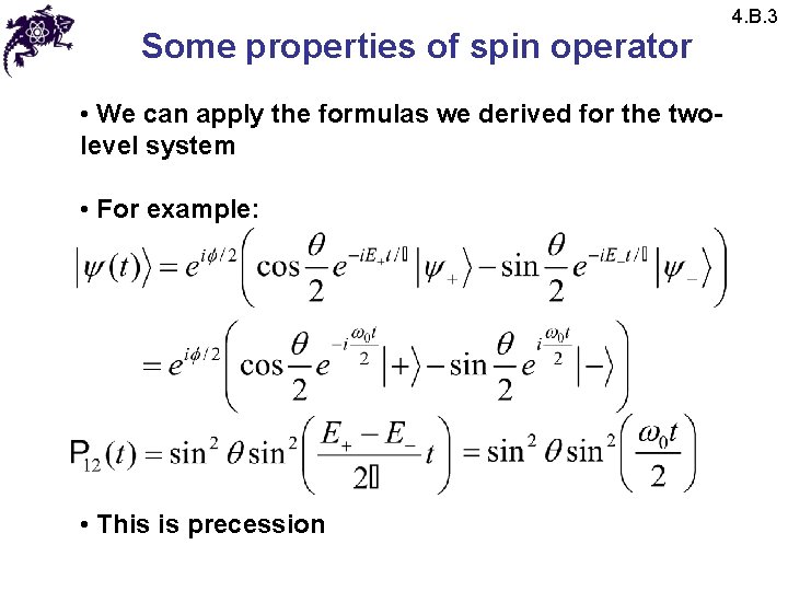
Some properties of spin operator • We can apply the formulas we derived for the twolevel system • For example: • This is precession 4. B. 3