Chapter 4 The Simplex Algorithm PART 2 Prof

Chapter 4 The Simplex Algorithm PART 2 Prof. Dr. M. Arslan ÖRNEK

2

ISE 203/IE 251 3

ISE 203/IE 251 4

ISE 203/IE 251 5

ISE 203/IE 251 6

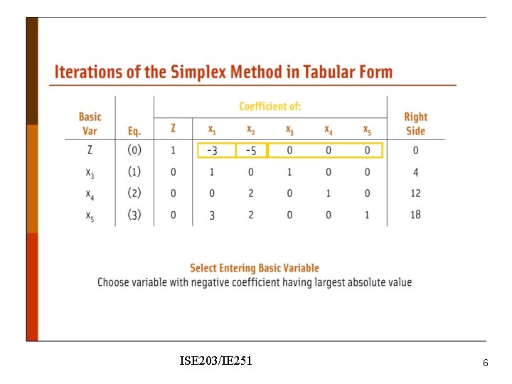
ISE 203/IE 251 7

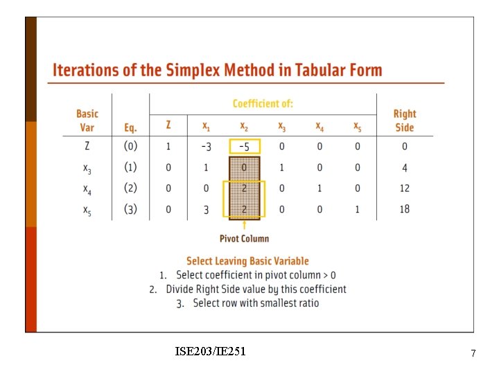
ISE 203/IE 251 8

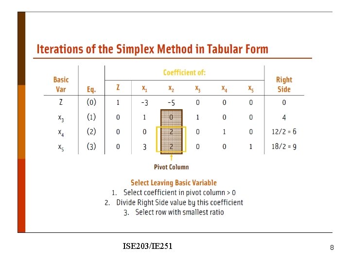
ISE 203/IE 251 9

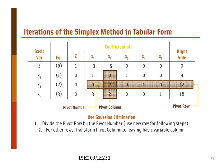
ISE 203/IE 251 10

ISE 203/IE 251 11

ISE 203/IE 251 12

ISE 203/IE 251 13

ISE 203/IE 251 14

ISE 203/IE 251 15

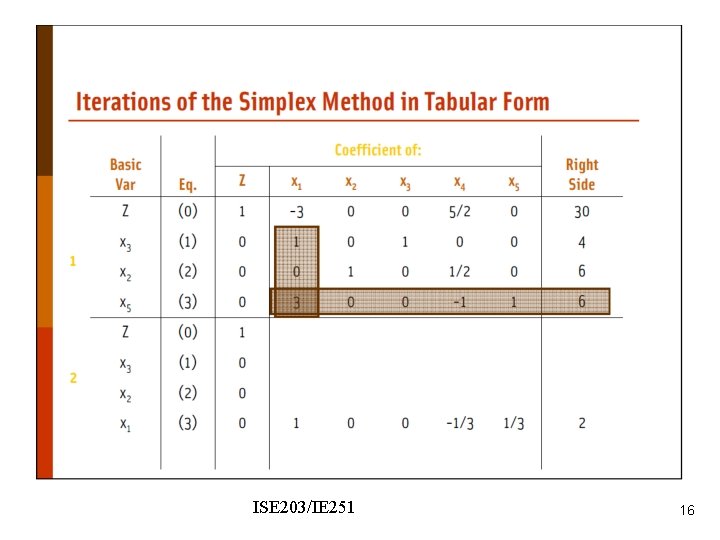
ISE 203/IE 251 16

ISE 203/IE 251 17

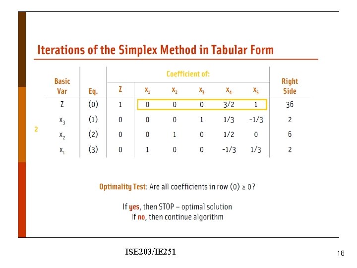
ISE 203/IE 251 18

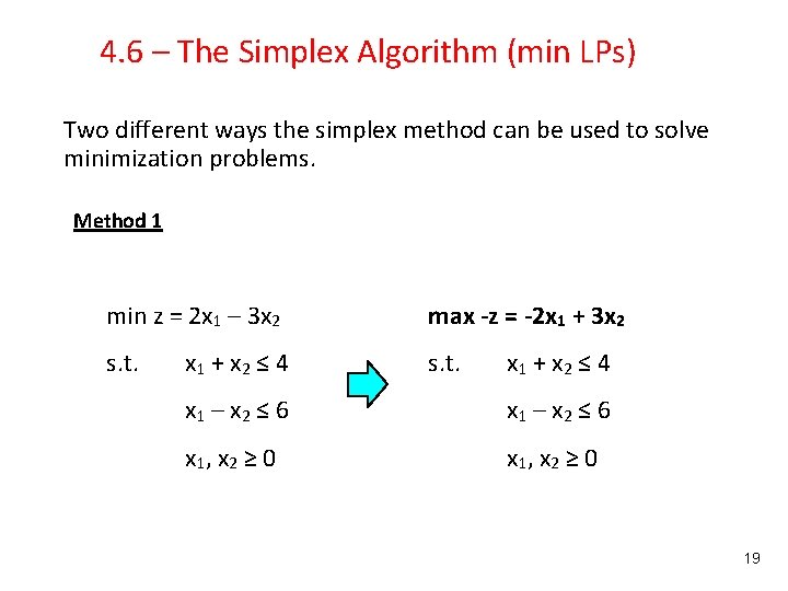
4. 6 – The Simplex Algorithm (min LPs) Two different ways the simplex method can be used to solve minimization problems. Method 1 min z = 2 x 1 – 3 x 2 max -z = -2 x 1 + 3 x 2 s. t. x 1 + x 2 ≤ 4 x 1 – x 2 ≤ 6 x 1 , x 2 ≥ 0 19

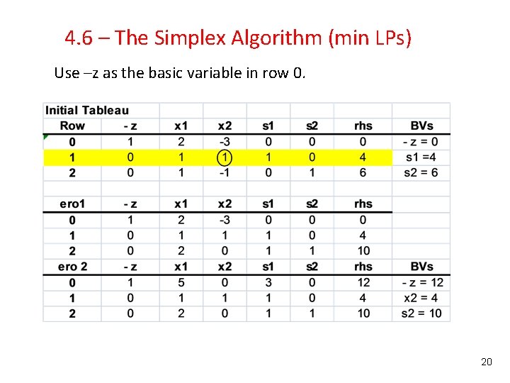
4. 6 – The Simplex Algorithm (min LPs) Use –z as the basic variable in row 0. 20

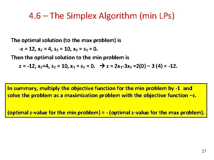
4. 6 – The Simplex Algorithm (min LPs) The optimal solution (to the max problem) is -z = 12, x 2 = 4, s 2 = 10, x 1 = s 1 = 0. Then the optimal solution to the min problem is z = -12, x 2=4, s 2 = 10, x 1 = s 2 = 0. z = 2 x 1 -3 x 2 =2(0) – 3 (4) = -12. In summary, multiply the objective function for the min problem by -1 and solve the problem as a maximization problem with the objective function –z. (optimal z-value for the min problem) = - (optimal z-value for the max problem). 21

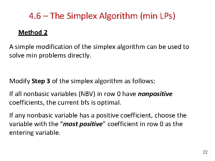
4. 6 – The Simplex Algorithm (min LPs) Method 2 A simple modification of the simplex algorithm can be used to solve min problems directly. Modify Step 3 of the simplex algorithm as follows: If all nonbasic variables (NBV) in row 0 have nonpositive coefficients, the current bfs is optimal. If any nonbasic variable has a positive coefficient, choose the variable with the “most positive” coefficient in row 0 as the entering variable. 22

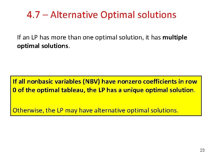
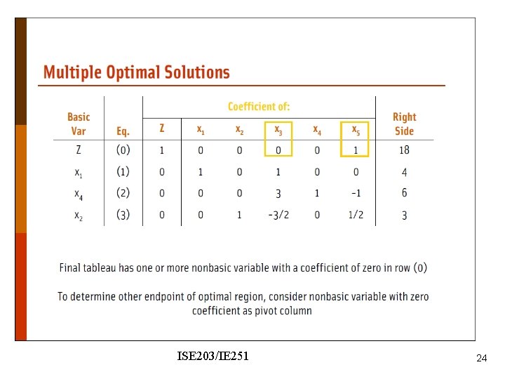
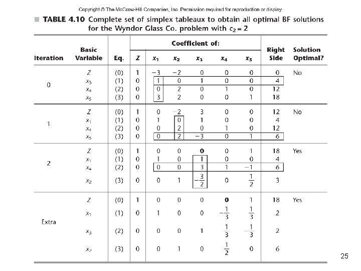
4. 7 – Alternative Optimal solutions If an LP has more than one optimal solution, it has multiple optimal solutions. If all nonbasic variables (NBV) have nonzero coefficients in row 0 of the optimal tableau, the LP has a unique optimal solution. Otherwise, the LP may have alternative optimal solutions. 23

ISE 203/IE 251 24

25

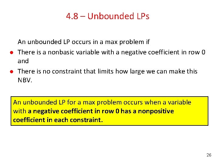
4. 8 – Unbounded LPs l l An unbounded LP occurs in a max problem if There is a nonbasic variable with a negative coefficient in row 0 and There is no constraint that limits how large we can make this NBV. An unbounded LP for a max problem occurs when a variable with a negative coefficient in row 0 has a nonpositive coefficient in each constraint. 26

ISE 203/IE 251 27

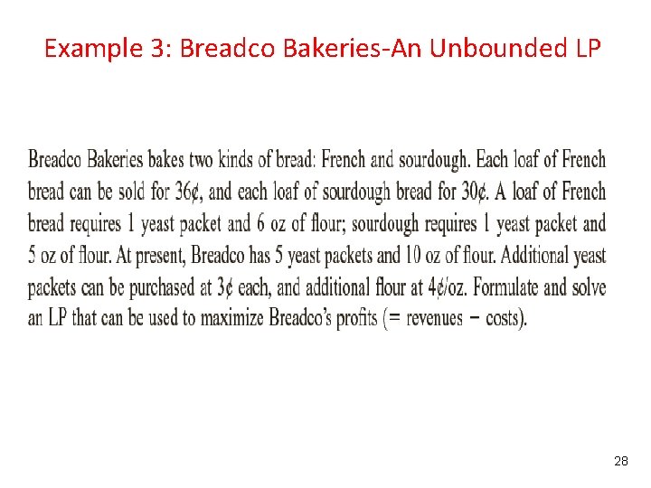
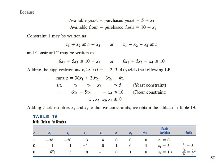
Example 3: Breadco Bakeries-An Unbounded LP 28

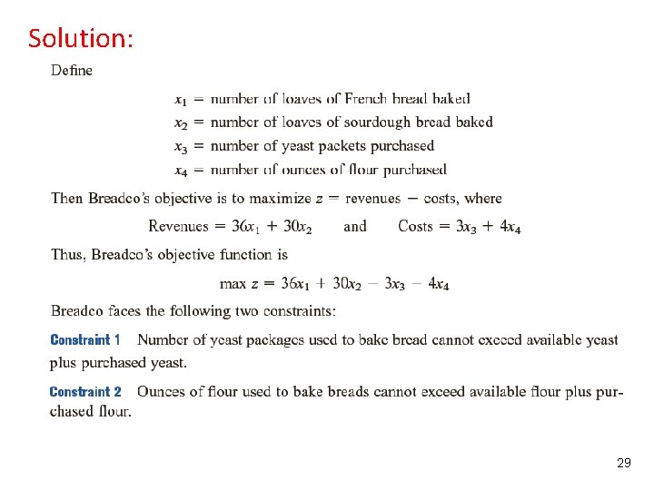
Solution: 29

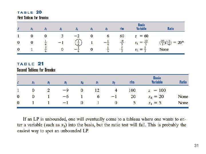
30

31

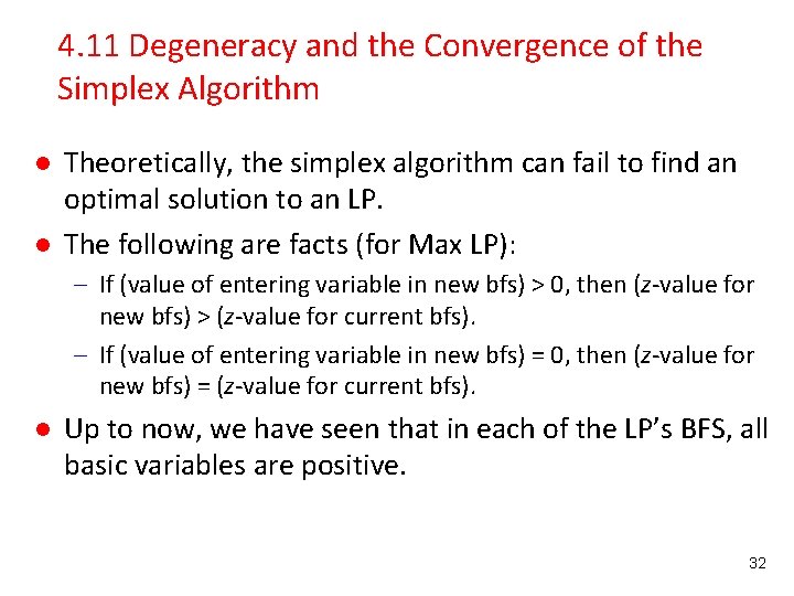
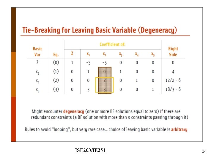
4. 11 Degeneracy and the Convergence of the Simplex Algorithm l l Theoretically, the simplex algorithm can fail to find an optimal solution to an LP. The following are facts (for Max LP): – If (value of entering variable in new bfs) > 0, then (z-value for new bfs) > (z-value for current bfs). – If (value of entering variable in new bfs) = 0, then (z-value for new bfs) = (z-value for current bfs). l Up to now, we have seen that in each of the LP’s BFS, all basic variables are positive. 32

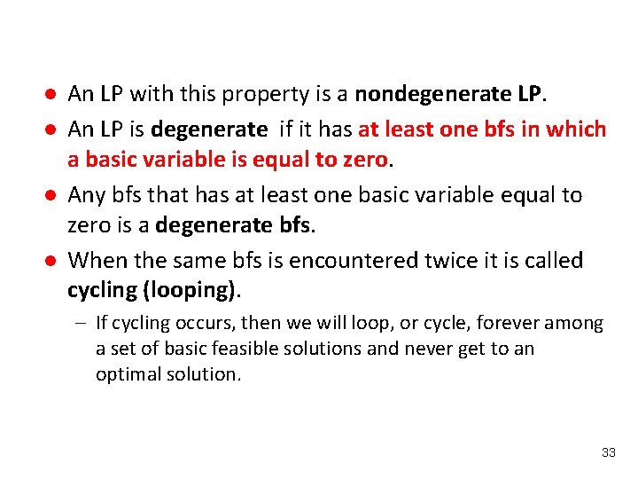
l l An LP with this property is a nondegenerate LP. An LP is degenerate if it has at least one bfs in which a basic variable is equal to zero. Any bfs that has at least one basic variable equal to zero is a degenerate bfs. When the same bfs is encountered twice it is called cycling (looping). – If cycling occurs, then we will loop, or cycle, forever among a set of basic feasible solutions and never get to an optimal solution. 33

ISE 203/IE 251 34

4. 12 The Big M Method l l The simplex algorithm requires a starting (initial) bfs. Previous problems have found starting bfs by using the slack variables as our basic variables. – If an LP have ≥ or = constraints, however, a starting bfs cannot be found easily. l In such a case, the Big M method is used to obtain a starting bfs and solve the problem. 35

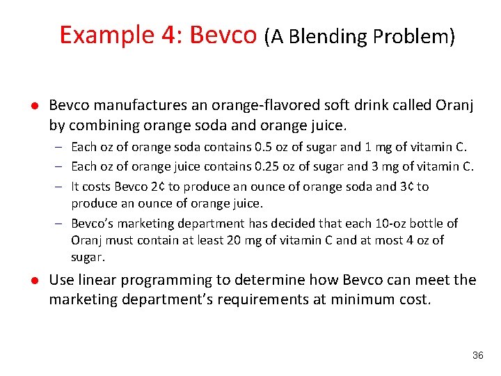
Example 4: Bevco (A Blending Problem) l Bevco manufactures an orange-flavored soft drink called Oranj by combining orange soda and orange juice. – Each oz of orange soda contains 0. 5 oz of sugar and 1 mg of vitamin C. – Each oz of orange juice contains 0. 25 oz of sugar and 3 mg of vitamin C. – It costs Bevco 2¢ to produce an ounce of orange soda and 3¢ to produce an ounce of orange juice. – Bevco’s marketing department has decided that each 10 -oz bottle of Oranj must contain at least 20 mg of vitamin C and at most 4 oz of sugar. l Use linear programming to determine how Bevco can meet the marketing department’s requirements at minimum cost. 36

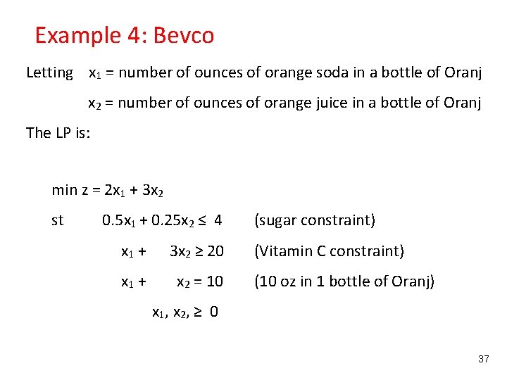
Example 4: Bevco Letting x 1 = number of ounces of orange soda in a bottle of Oranj x 2 = number of ounces of orange juice in a bottle of Oranj The LP is: min z = 2 x 1 + 3 x 2 st 0. 5 x 1 + 0. 25 x 2 ≤ 4 x 1 + 3 x 2 ≥ 20 x 1 + x 2 = 10 (sugar constraint) (Vitamin C constraint) (10 oz in 1 bottle of Oranj) x 1, x 2, ≥ 0 37

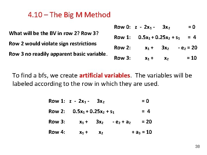
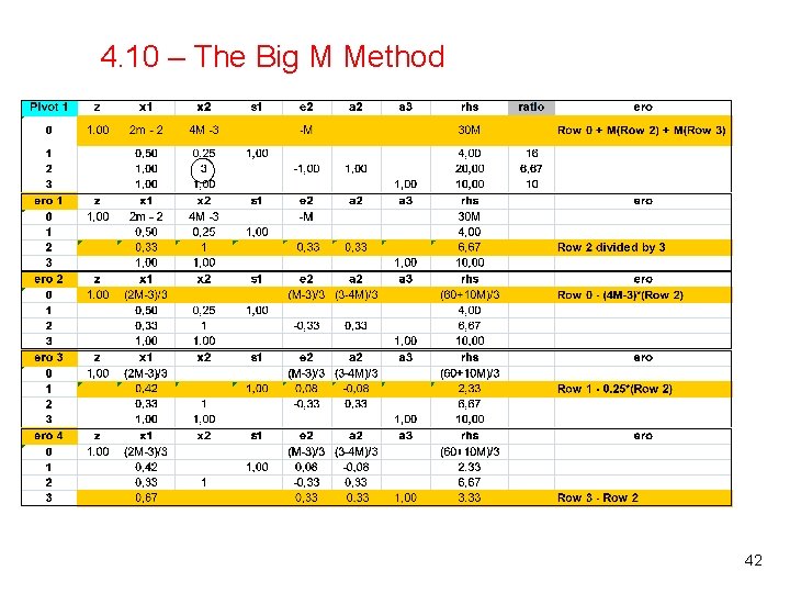
4. 10 – The Big M Method What will be the BV in row 2? Row 3? Row 2 would violate sign restrictions Row 3 no readily apparent basic variable. Row 0: z - 2 x 1 Row 1: 3 x 2 =0 0. 5 x 1 + 0. 25 x 2 + s 1 = 4 Row 2: x 1 + 3 x 2 - e 2 = 20 Row 3: x 1 + x 2 = 10 To find a bfs, we create artificial variables. The variables will be labeled according to the row in which they are used. Row 1: z - 2 x 1 Row 2: 3 x 2 =0 0. 5 x 1 + 0. 25 x 2 + s 1 Row 3: x 1 + 3 x 2 Row 4: x 1 + x 2 - e 2 + a 2 = 4 = 20 + a 3 = 10 38

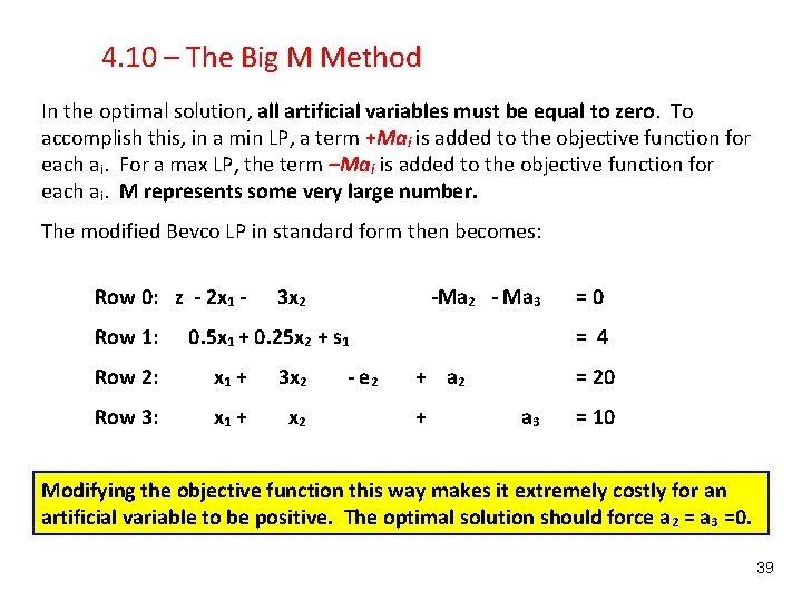
4. 10 – The Big M Method In the optimal solution, all artificial variables must be equal to zero. To accomplish this, in a min LP, a term +Mai is added to the objective function for each ai. For a max LP, the term –Mai is added to the objective function for each ai. M represents some very large number. The modified Bevco LP in standard form then becomes: Row 0: z - 2 x 1 Row 1: 3 x 2 -Ma 2 - Ma 3 0. 5 x 1 + 0. 25 x 2 + s 1 Row 2: x 1 + 3 x 2 Row 3: x 1 + x 2 - e 2 =0 = 4 + a 2 + = 20 a 3 = 10 Modifying the objective function this way makes it extremely costly for an artificial variable to be positive. The optimal solution should force a 2 = a 3 =0. 39

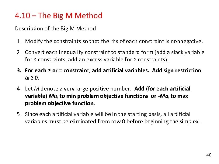
4. 10 – The Big M Method Description of the Big M Method: 1. Modify the constraints so that the rhs of each constraint is nonnegative. 2. Convert each inequality constraint to standard form (add a slack variable for ≤ constraints, add an excess variable for ≥ constraints). 3. For each ≥ or = constraint, add artificial variables. Add sign restriction ai ≥ 0. 4. Let M denote a very large positive number. Add (for each artificial variable) Mai to min problem objective functions or -Mai to max problem objective function. 5. Since each artificial variable will be in the starting basis, all artificial variables must be eliminated from row 0 before beginning the simplex. 40

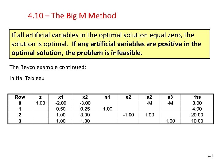
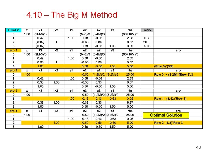
4. 10 – The Big M Method If all artificial variables in the optimal solution equal zero, the solution is optimal. If any artificial variables are positive in the optimal solution, the problem is infeasible. The Bevco example continued: Initial Tableau 41

4. 10 – The Big M Method 42

4. 10 – The Big M Method 43

Wyndor Problem - modified ISE 203/IE 251 44

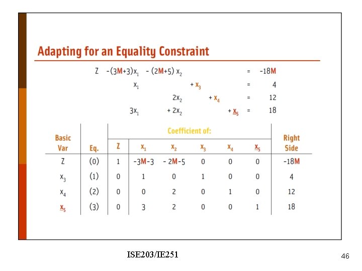
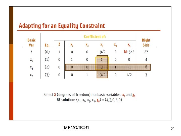
Nonzero coefficient of x 5 in the objective function row. We should make it zero. ISE 203/IE 251 45

ISE 203/IE 251 46

ISE 203/IE 251 47

ISE 203/IE 251 48

ISE 203/IE 251 49

ISE 203/IE 251 50

ISE 203/IE 251 51

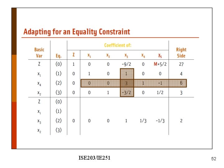
ISE 203/IE 251 52

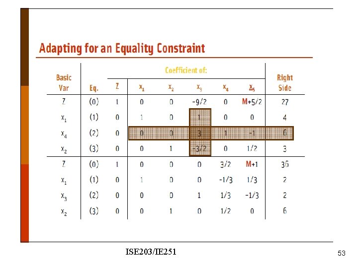
ISE 203/IE 251 53

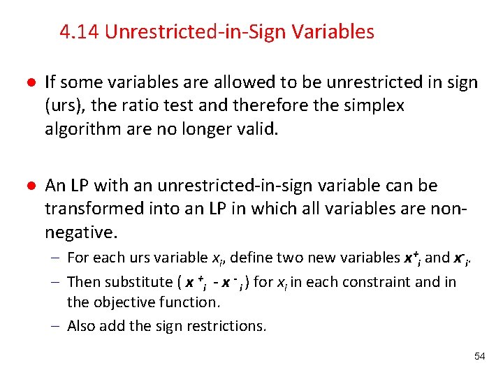
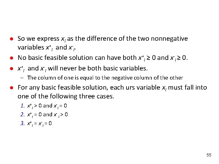
4. 14 Unrestricted-in-Sign Variables l If some variables are allowed to be unrestricted in sign (urs), the ratio test and therefore the simplex algorithm are no longer valid. l An LP with an unrestricted-in-sign variable can be transformed into an LP in which all variables are nonnegative. – For each urs variable xi, define two new variables x+i and x-i. – Then substitute ( x +i - x - i ) for xi in each constraint and in the objective function. – Also add the sign restrictions. 54

l l l So we express xi as the difference of the two nonnegative variables x+i and x-i. No basic feasible solution can have both x+i ≥ 0 and x-i ≥ 0. x+i and x-i will never be both basic variables. – The column of one is equal to the negative column of the other l For any basic feasible solution, each urs variable xi must fall into one of the following three cases. 1. x+i > 0 and x-i = 0 2. x+i = 0 and x- i > 0 3. x+i = x-i = 0 55

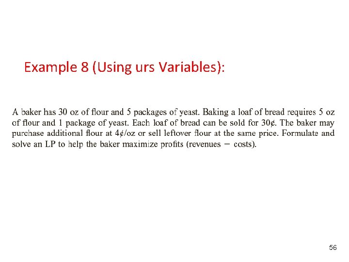
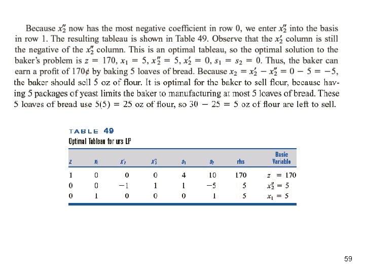
Example 8 (Using urs Variables): 56

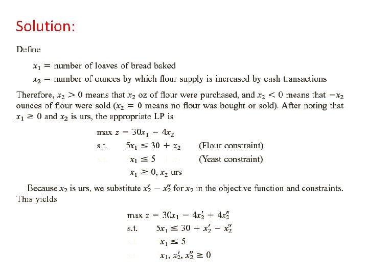
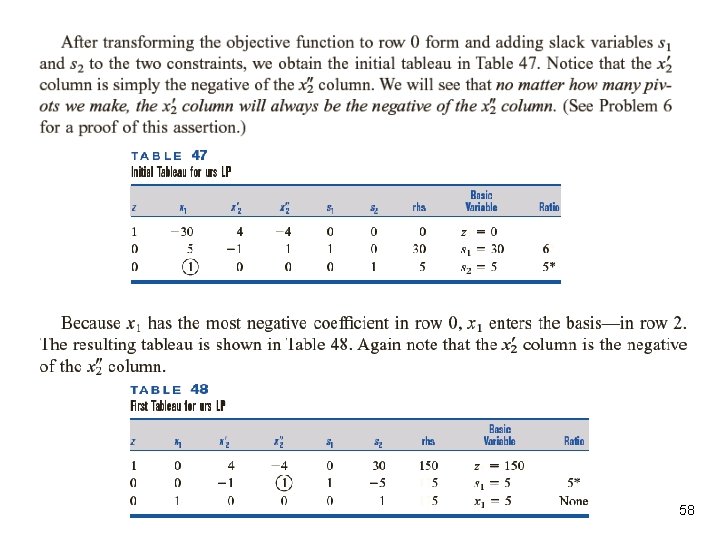
Solution: 57

58

59