Chapter 4 Systems of ODEs Phase Plane Qualitative

Chapter 4 Systems of ODEs. Phase Plane. Qualitative Methods 歐亞書局 P

Contents 4. 0 Basics of Matrices and Vectors 4. 1 Systems of ODEs as Models 4. 2 Basic Theory of Systems of ODEs 4. 3 Constant-Coefficient Systems. Phase Plane Method 4. 4 Criteria for Critical Points. Stability 4. 5 Qualitative Methods for Nonlinear Systems 4. 6 Nonhomogeneous Linear Systems of ODEs Summary of Chapter 4 歐亞書局 P

4. 1 Systems of ODEs as Models Example 1 Mixing Problem Involving Two Tanks A mixing problem involving a single tank can be modeled by a single ODE. The model will be a system of two firstorder ODEs. Tank T 1 and T 2 in Fig. 77 contain initially 100 gal of water each. In T 1 the water is pure, whereas 150 lb of fertilizer are dissolved in T 2. By circulating liquid at a rate of 2 gal/min and stirring (to keep the mixture uniform) the amounts of fertilizer y 1(t) in T 1 and y 2(t) in T 2 change with time t. How long should we let the liquid circulate so that T 1 will contain at least half as much fertilizer as there will be left in T 2? continued 歐亞書局 P 130

Fig. 77. Fertilizer content in Tanks T 1 (lower curve) and T 2 (upper curve) continued 歐亞書局 P 131

Solution. Step 1. Setting up the model. As for a single tank, the time rate of change y'1(t) of y 1(t) equals inflow minus outflow. Similarly for tank T 2. From Fig. 77 we see that Hence the mathematical model of our mixture problem is the system of first-order ODEs 歐亞書局 P 130 y'1 = – 0. 02 y 1 + 0. 02 y 2 (Tank T 1) y'2 = 0. 02 y 1 – 0. 02 y 2 (Tank T 2). continued

As a vector equation with column vector y = this becomes and matrix A Step 2. General solution. As for a single equation, we try an exponential function of t, (1) y = xeλt. Then y' = λxeλt = Axeλt. Dividing the last equation λxeλt = Axeλt by eλt and interchanging the left and right sides, we obtain Ax = λx continued 歐亞書局 P 131

Since nontrivial solutions are needed, we have to look for eigenvalues and eigenvectors of A. The eigenvalues are the solutions of the characteristic equation (2) We see that λ 1 = 0 and λ 2 = – 0. 04. For our present A this gives a) – 0. 02 x 1 + 0. 02 x 2 = 0 (λ 1 = 0) b) (– 0. 02 + 0. 04)x 1 + 0. 02 x 2 = 0 (λ 2 = – 0. 04) continued 歐亞書局 P 131

Hence x 1 = x 2 (λ 1 = 0) and x 1 = –x 2 (λ 2 = – 0. 04), respectively, and we can take x 1 = x 2 = 1 and x 1 = –x 2 = 1. This gives two eigenvectors corresponding to λ 1 = 0 and λ 2 = – 0. 04, respectively, namely, From (1) and the superposition principle, we thus obtain a solution (3) where c 1 and c 2 are arbitrary constants. Later we shall call this a general solution. continued 歐亞書局 P 131

Step 3. Use of initial conditions. The initial conditions are y 1(0) = 0 (no fertilizer in tank T 1) and y 2(0) = 150. From this and (3) with t = 0 we obtain In components this is c 1 + c 2 = 0, c 1 – c 2 = 150. The solution is c 1 = 75, c 2 = – 75. This gives the answer ∴ y 1 = 75 – 75 e-0. 04 t; y 2 = 75 + 75 e-0. 04 t Figure 77 shows the exponential increase of y 1 and the exponential decrease of y 2 to the common limit 75 lb. continued 歐亞書局 P 131

Step 4. Answer. T 1 contains half the fertilizer amount of T 2 if it contains 1/3 of the total amount, that is, 50 lb. Thus y 1 = 75 – 75 e-0. 04 t = 50, t = (ln 3)/0. 04 = 27. 5. 歐亞書局 P 132 e-0. 04 t = 1/3,

8. 4 Eigenbases. Diagonalization. Quadratic Forms Theorem 4 Diagonalization of a Matrix If an n × n matrix A has a basis of eigenvectors, then (5) D = X− 1 AX is diagonal, with the eigenvalues of A as the entries on the main diagonal. Here X is the matrix with these eigenvectors as column vectors. Also, (5*) Section 8. 4 p 11 歐亞書局 P Dm = X− 1 Am. X (m = 2, 3, … ).

Generalized Formulation 歐亞書局 P

Eigen Values Eigenvectors 歐亞書局 P

Nonhomogeneous Equations The nonhomogeneous equation y' + p(x) y = r(x) 歐亞書局 P

Example 2 Electrical Network continued 歐亞書局 P 132

Solution. Step 1. Setting up the mathematical model. The model of this network is obtained from Kirchhoff’s voltage law, as in Sec. 2. 9 (where we considered single circuits). Let I 1(t) and I 2(t) be the currents in the left and right loops, respectively. In the left loop the voltage drops are LI'1 = I'1 [V] over the inductor and R 1(I 1 – I 2) = 4(I 1 – I 2) [V] over the resistor, the difference because I 1 and I 2 flow through the resistor in opposite directions. By Kirchhoff’s voltage law the sum of these drops equals the voltage of the battery; that is, I'1 + 4(I 1 – I 2) = 12, hence (4 a) I'1 = – 4 I 1 + 4 I 2 + 12. continued 歐亞書局 P 132

In the right loop the voltage drops are R 2 I 2 = 6 I 2 [V] and R 1(I 2 – I 1) = 4(I 2 – I 1) [V] over the resistors and (1/C)∫I 2 dt = 4∫I 2 dt [V] over the capacitor, and their sum is zero, Division by 10 and differentiation gives I'2 – 0. 4 I'1 + 0. 4 I 2 = 0. To simplify the solution process, we first get rid of 0. 4 I'1, which by (4 a) equals 0. 4(– 4 I 1 + 4 I 2 + 12). Substitution into the present ODE gives I'2 = 0. 4 I'1 – 0. 4 I 2 = 0. 4(– 4 I 1 + 4 I 2 + 12) – 0. 4 I 2 continued 歐亞書局 P 132

and by simplification (4 b) I'2 = – 1. 6 I 1 + 1. 2 I 2 + 4. 8. In matrix form, (4) is (we write J since I is the unit matrix) (5) Step 2. Solving (5). Because of the vector g this is a nonhomogeneous system. We try to proceed as for a single ODE, solving first the homogeneous system J' = AJ by substituting J = xeλt J' = xeλt = Axeλt ∴ Ax =λx. 歐亞書局 P 133 continued

Hence to obtain a nontrivial solution, we again need the eigenvalues and eigenvectors: Hence a “general solution” of the homogeneous system is Jh = c 1 x(1)e-2 t + c 2 x(2)e-0. 8 t. For a particular solution of the nonhomogeneous system (5), since g is constant, we try a constant column vector Jp = a with components a 1, a 2. Then J'p = 0, and substitution into (5) gives continued 歐亞書局 P 133

– 4. 0 a 1 + 4. 0 a 2 + 12. 0 = 0 – 1. 6 a 1 + 1. 2 a 2 + 4. 8 = 0. The solution is a 1 = 3, a 2 = 0; thus a = (6) . Hence J = Jh + Jp = c 1 x(1)e-2 t + c 2 x(2)e-0. 8 t + a; in components, I 1 = 2 c 1 e-2 t + c 2 e-0. 8 t + 3 I 2 = c 1 e-2 t + 0. 8 c 2 e-0. 8 t. 歐亞書局 P 133 continued

The initial conditions give I 1(0) = 2 c 1 + c 2 + 3 = 0 I 2(0) = c 1 + 0. 8 c 2 = 0. Hence c 1 = – 4 and c 2 = 5. As the solution of our problem we thus obtain (7) J = – 4 x(1)e-2 t + 5 x(2)e-0. 8 t + a. In components (Fig. 79 b), I 1 = – 8 e-2 t + 5 e-0. 8 t + 3 I 2 = – 4 e-2 t + 4 e-0. 8 t. 歐亞書局 P 133 continued

Fig. 79. Currents in Example 2 歐亞書局 P 134

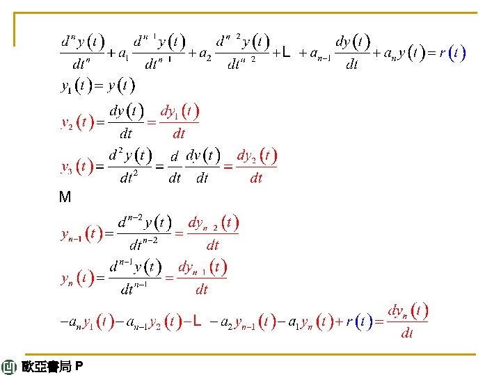
Conversion of an nth-Order ODE to a System THEOREM 1 Conversion of an ODE An nth-order ODE (8) can be converted to a system of n first-order ODEs by setting (9) y 1 = y, y 2 = y', y 3 = y'', ‥‥ , yn = y(n– 1). This system is of the form (10) 歐亞書局 P 134

Example 3 Mass on a Spring Let us consider the free motions of a mass on a spring For this ODE (8) the system (10) is linear and homogeneous, continued 歐亞書局 P 135

Setting y = , we get in matrix form The characteristic equation is For an illustrative computation, let m = 1, c = 2, and k = 0. 75: λ 2 + 2λ+ 0. 75 = (λ+ 0. 5)(λ+ 1. 5) = 0. This gives the eigenvalues λ 1 = – 0. 5 and λ 2 = – 1. 5. continued 歐亞書局 P 135

Eigenvectors follow from the first equation in A – λI = 0, which is –λx 1 + x 2 = 0. For λ 1 this gives 0. 5 x 1 + x 2 = 0, say, x 1 = 2, x 2 = – 1. For λ 2 = – 1. 5 it gives 1. 5 x 1 + x 2 = 0, say, x 1 = 1, x 2 = – 1. 5. These eigenvectors This vector solution has the first component y = y 1 = 2 c 1 e-0. 5 t + c 2 e-1. 5 t which is the expected solution. The second component is its derivative y 2 = y'1 = y' = –c 1 e-0. 5 t – 1. 5 c 2 e-1. 5 t. 歐亞書局 P 135

Phase Variable Canonical Form 歐亞書局 P

Vandermonde Matrix 歐亞書局 P

Example 歐亞書局 P

4. 3 Constant-Coefficient Systems. Phase Plane Method THEOREM 1 General Solution If the constant matrix A in the system (1) has a linearly independent set of n eigenvectors, then the corresponding solutions y(1), ‥‥, y(n) in (4) form a basis of solutions of (1), and the corresponding general solution is (5) 歐亞書局 P 140

How to Graph Solutions in the Phase Plane We shall now concentrate on systems (1) with constant coefficients consisting of two ODEs y'1 = a 11 y 1 + a 12 y 2 (6) y' = Ay; in components, y'2 = a 21 y 1 + a 22 y. Of course, we can graph solutions of (6), (7) continued 歐亞書局 P 140

as two curves over the t-axis, one for each component of y(t). (Figure 79 a in Sec. 4. 1 shows an example. ) But we can also graph (7) as a single curve in the y 1 y 2 -plane. This is a parametric representation (parametric equation) with parameter t. (See Fig. 79 b for an example. Many more follow. Parametric equations also occur in calculus. ) Such a curve is called a trajectory (or sometimes an orbit or path) of (6). The y 1 y 2 -plane is called the phase plane. If we fill the phase plane with trajectories of (6), we obtain the socalled phase portrait of (6). 歐亞書局 P 141

E X A M P L E 1 Trajectories in the Phase Plane (Phase Portrait) In order to see what is going on, let us find and graph solutions of the system (8) Solution. By substituting y = xeλt and y' = xeλt and dropping the exponential function we get Ax = λx. The characteristic equation is This gives the eigenvalues λ 1 = – 2 and λ 2 = – 4. Eigenvectors are then obtained from (– 3 – λ)x 1 + x 2 = 0. 歐亞書局 P 141 continued

For λ 1 = – 2 this is –x 1 + x 2 = 0. Hence we can take x(1) = [1 1]T. For λ 2 = – 4 this becomes x 1 + x 2 = 0, and an eigenvector is x(2) = [1 – 1]T. This gives the general solution Figure 81 shows a phase portrait of some of the trajectories (to which more trajectories could be added if so desired). The two straight trajectories correspond to c 1 = 0 and c 2 = 0 and the others to other choices of c 1, c 2. 歐亞書局 P 141

Critical Points of the System (6) The point y = 0 in Fig. 81 seems to be a common point of all trajectories, and we want to explore the reason for this remarkable observation. The answer will follow by calculus. Indeed, from (6) we obtain (9) This associates with every point P: (y 1, y 2) a unique tangent direction dy 2/dy 1 of the trajectory passing through P, except for the point P = P 0: (0, 0), where the right side of (9) becomes 0/0. This point P 0, at which dy 2/dy 1 becomes undetermined, is called a critical point of (6). 歐亞書局 P 141

Five Types of Critical Points E X A M P L E 1 (Continued) Improper Node (Fig. 81) An improper node is a critical point P 0 at which all the trajectories, except for two of them, have the same limiting direction of the tangent. The two exceptional trajectories also have a limiting direction of the tangent at P 0 which, however, is different. The system (8) has an improper node at 0, as its phase portrait Fig. 81 shows. The common limiting direction at 0 is that of the eigenvector x(1) = [1 1]T because e-4 t goes to zero faster than e-2 t as t increases. The two exceptional limiting tangent directions are those of x(2) = [1 – 1]T and –x(2) = [– 1 1]T. continued 歐亞書局 P 142

Fig. 81. Trajectories of the system (8) (Improper node) 歐亞書局 P 142

E X A M P L E 2 Proper Node (Fig. 82) A proper node is a critical point P 0 at which every trajectory has a definite limiting direction and for any given direction d at P 0 there is a trajectory having d as its limiting direction. The system (10) continued 歐亞書局 P 142

has a proper node at the origin (see Fig. 82). Indeed, the matrix is the unit matrix. Its characteristic equation (1 –λ)2 = 0 has the root λ = 1. Any x ≠ 0 is an eigenvector, and we can take [1 0]T and [0 1]T. Hence a general solution is continued 歐亞書局 P 142

Fig. 82. Trajectories of the system (10) (Proper node) 歐亞書局 P 142

E X A M P L E 3 Saddle Point (Fig. 83) A saddle point is a critical point P 0 at which there are two incoming trajectories, two outgoing trajectories, and all the other trajectories in a neighborhood of P 0 bypass P 0. The system (11) continued 歐亞書局 P 143

has a saddle point at the origin. Its characteristic equation (1 –λ)(– 1 –λ) = 0 has the roots λ 1 = 1 and λ 2 = – 1. For λ 1= 1 an eigenvector [1 0]T is obtained from the second row of (A –λI)x = 0, that is, 0 x 1 + (– 1 – 1)x 2 = 0. For λ 2 = – 1 the first row gives [0 1]T. Hence a general solution is This is a family of hyperbolas (and the coordinate axes); see Fig. 83. continued 歐亞書局 P 143

Fig. 83. Trajectories of the system (11) (Saddle point) 歐亞書局 P 143

E X A M P L E 4 Center (Fig. 84) A center is a critical point that is enclosed by infinitely many closed trajectories. The system (12) has a center at the origin. The characteristic equation λ 2 + 4 = 0 gives the eigenvalues 2 i and – 2 i. For 2 i an eigenvector follows from the first equation – 2 ix 1 + x 2 = 0 of (A –λI)x = 0, say, [1 2 i]T. For λ = – 2 i that equation is –(– 2 i)x 1 + x 2 = 0 and gives, say, [1 – 2 i]T. Hence a complex general solution is (12*) 歐亞書局 P 143 continued

The next step would be the transformation of this solution to real form by the Euler formula (Sec. 2. 2). But we were just curious to see what kind of eigenvalues we obtain in the case of a center. Accordingly, we do not continue, but start again from the beginning and use a shortcut. We rewrite the given equations in the form y'1 = y 2, 4 y 1 = –y'2; then the product of the left sides must equal the product of the right sides, This is a family of ellipses (see Fig. 84) enclosing the center at the origin. continued 歐亞書局 P 143

Fig. 84. Trajectories of the system (12) (Center) 歐亞書局 P 143

E X A M P L E 5 Spiral Point (Fig. 85) A spiral point is a critical point P 0 about which the trajectories spiral, approaching P 0 as t → ∞(or tracing these spirals in the opposite sense, away from P 0). The system (13) continued 歐亞書局 P 144

has a spiral point at the origin, as we shall see. The characteristic equation is λ 2 + 2λ+ 2 = 0. It gives the eigenvalues – 1 + i and – 1 – I. Corresponding eigenvectors are obtained from (– 1 –λ)x 1 + x 2 = 0. For λ = – 1 + i this becomes –ix 1 + x 2 = 0 and we can take [1 i]T as an eigenvector. Similarly, an eigenvector corresponding to – 1 – i is [1 –i]T. This gives the complex general solution continued 歐亞書局 P 144

The next step would be the transformation of this complex solution to a real general solution by the Euler formula. But, as in the last example, we just wanted to see what eigenvalues to expect in the case of a spiral point. Accordingly, we start again from the beginning and instead of that rather lengthy systematic calculation we use a shortcut. We multiply the first equation in (13) by y 1, the second by y 2, and add, obtaining y 1 y'1 + y 2 y'2 = –(y 12 + y 22). continued 歐亞書局 P 144

We now introduce polar coordinates r, t, where r 2 = y 12 + y 22. Differentiating this with respect to t gives 2 rr' = 2 y 1 y'1 + 2 y 2 y'2. Hence the previous equation can be written rr' = –r 2, Thus, r' = –r, dr/r = –dt, ln│r│ = –t + c*, r = ce-t. For each real c this is a spiral, as claimed. (see Fig. 85). continued 歐亞書局 P 144

Fig. 85. Trajectories of the system (13) (Spiral point) 歐亞書局 P 144

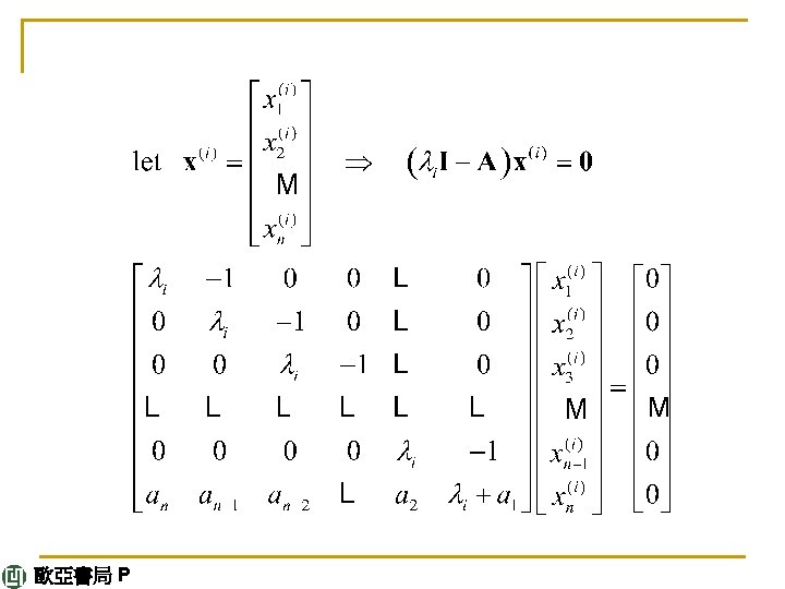
E X A M P L E 6 No Basis of Eigenvectors Available. Degenerate Node (Fig. 86) This cannot happen if A in (1) is symmetric (akj = ajk, as in Examples 1– 3) or skew-symmetric (akj = –ajk, thus ajj = 0). And it does not happen in many other cases (see Examples 4 and 5). Hence it suffices to explain the method to be used by an example. Find and graph a general solution of (14) continued 歐亞書局 P 144

Solution. A is not skew-symmetric! Its characteristic equation is It has a double root λ= 3. Hence eigenvectors are obtained from (4 –λ)x 1 + x 2 = 0, thus from x 1 + x 2 = 0, say, x(1) = [1 – 1]T and nonzero multiples of it (which do not help). The method now is to substitute y(2) = xteλt + ueλt continued 歐亞書局 P 145

with constant u = [u 1 u 2]T into (14). (The xt-term alone, the analog of what we did in Sec. 2. 2 in the case of a double root, would not be enough. Try it. ) This gives y'(2) = xeλt + λxteλt + λueλt = Ay(2) = Axteλt + Aueλt. On the right, Ax = λx. Hence the terms λxteλt cancel, and then division by eλt gives x +λu = Au, thus (A –λI)u = x. Here λ= 3 and x = [1 – 1]T, so that 歐亞書局 P 145 continued

A solution, linearly independent of x = [1 – 1]T, is u = [0 1]T. This yields the answer (Fig. 86) The critical point at the origin is often called a degenerate node. c 1 y(1) gives the heavy straight line, with c 1 > 0 the lower part and c 1 < 0 the upper part of it. y(2) gives the right part of the heavy curve from 0 through the second, first, and—finally—fourth quadrants. –y(2) gives the other part of that curve. continued 歐亞書局 P 145

Fig. 86. Degenerate node in Example 6 歐亞書局 P 145

4. 4 Criteria for Critical Points. Stability We continue our discussion of homogeneous linear systems with constant coefficients (1) 歐亞書局 P 147

(3) We also recall from Sec. 4. 3 that there are various types of critical points, and we shall now see how these types are related to the eigenvalues. The latter are solutions λ=λ 1 and λ 2 of the characteristic equation (4) continued 歐亞書局 P 147

This is a quadratic equation λ 2 – pλ + q = 0 with coefficients p, q and discriminant Δ given by (5) p = a 11 + a 22, q = det A = a 11 a 22 – a 12 a 21, Δ = p 2 – 4 q. From calculus we know that the solutions of this equation are (6) 歐亞書局 P 147

Table 4. 1 Eigenvalue Criteria for Critical Points (Derivation after Table 4. 2) 歐亞書局 P 148

Stability DEFINITION Stable, Unstable, Stable and Attractive(1) A critical point P 0 of (1) is called stable if, roughly, all trajectories of (1) that at some instant are close to P 0 remain close to P 0 at all future times; precisely: if for every disk Dε of radius ε< 0 with center P 0 there is a disk Dδ of radius δ > 0 with center P 0 such that every trajectory of (1) that has a point P 1 (corresponding to t = t 1, say) in Dδ has all its points corresponding to t ≥ t 1 in Dε. See Fig. 89. continued 歐亞書局 P 148

DEFINITION Stable, Unstable, Stable and Attractive(2) P 0 is called unstable if P 0 is not stable. P 0 is called stable and attractive (or asymptotically stable) if P 0 is stable and every trajectory that has a point in Dδ approaches P 0 as t →∞. See Fig. 90. 歐亞書局 P 148

Fig. 89. Stable critical point P 0 of (1) (The trajectory initiating at P 1 stays in the disk of radius ε. ) 歐亞書局 P 149

Fig. 90. Stable and attractive critical point P 0 of (1) 歐亞書局 P 149

Table 4. 2 Stability Criteria for Critical Points 歐亞書局 P 149

E X A M P L E 1 Application of the Criteria in Tables 4. 1 and 4. 2 In Example 1, Sec. 4. 3, we have y' = y, p = – 6, q = 8, Δ = 4, a node by Table 4. 1(a), which is stable and attractive by Table 4. 2(a). 歐亞書局 P 149

E X A M P L E 2 Free Motions of a Mass on a Spring What kind of critical point does my" + cy' + ky = 0 in Sec. 2. 4 have? Solution. Division by m gives y'' = –(k/m)y – (c/m)y'. To get a system, set y 1 = y, y 2 = y' (see Sec. 4. 1). Then y'2 = y'' = –(k/m)y 1 – (c/m)y 2. Hence continued 歐亞書局 P 150

We see that p = –c/m, q = k/m, Δ = (c/m)2 – 4 k/m. From this and Tables 4. 1 and 4. 2 we obtain the following results. Note that in the last three cases the discriminant Δ plays an essential role. No damping. c = 0, p = 0, q > 0, a center. Underdamping. c 2 < 4 mk, p < 0, q > 0, Δ < 0, a stable and attractive spiral point. Critical damping. c 2 = 4 mk, p < 0, q > 0, Δ = 0, a stable and attractive node. Overdamping. c 2 > 4 mk, p < 0, q > 0, Δ > 0, a stable and attractive node. 歐亞書局 P 150

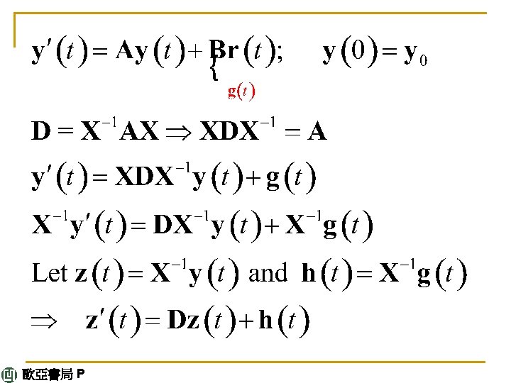
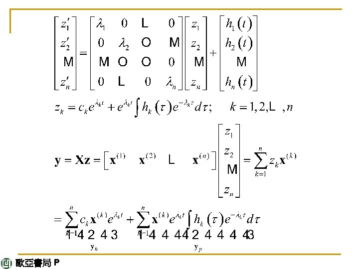
4. 6 Nonhomogeneous Linear Systems of ODEs In this last section of Chap. 4 we discuss methods for solving nonhomogeneous linear systems of ODEs (1) y' = Ay + g where the vector g(t) is not identically zero. We assume g(t) and the entries of the n × n matrix A(t) to be continuous on some interval J of the t-axis. continued 歐亞書局 P 159

From a general solution y(h)(t) of the homogeneous system y'= Ay and a particular solution y(p)(t) of (1), we get (2) y = y(h) + y(p). where y is called a general solution of (1) because it includes every solution of (1). 歐亞書局 P 159

Method of Undetermined Coefficients As for a single ODE, this method is suitable if (1) the entries of A are constants and (2) the components of g are • constants, • positive integer powers of t, • exponential functions, or • cosines and sines. In such a case a particular solution y(p) is assumed in a form similar to g; for instance, y(p) = u + vt + wt 2 if g has components quadratic in t, with u, v, w to be determined by substitution into (1). This is similar to Sec. 2. 7, except for the Modification Rule. . 歐亞書局 P 160

Example 1 Method of Undetermined Coefficients. Modification Rule Find a general solution of (3) Solution. A general equation of the homogeneous system is (see Example 1 in Sec. 4. 3) Eigen values (4) Eigen vectors continued 歐亞書局 P 160

continued 歐亞書局 P 160

Equating the te-2 t-terms on both sides, we have – 2 u = Au Hence u must be an eigenvector of A corresponding to λ = – 2; thus u = a[1 1]T with any a ≠ 0. Equating the e-2 t-terms gives Collecting terms and reshuffling gives v 1 – v 2 = –a – 6 –v 1 + v 2 = –a + 2. 歐亞書局 P 160 continued

By addition, 0 = – 2 a – 4, a = – 2, ∴v 2 = v 1 + 4. Let v 1 = k v = [k k + 4]T We can simply choose k = 0. This gives 歐亞書局 P 160

Method of Variation of Parameters This method can be applied to nonhomogeneous linear systems (6) y' = A(t)y + g(t) with variable A = A(t) and general g(t). It yields a particular solution y(p) of (6) on some open interval J on the t-axis if a general solution of the homogeneous system y' = A(t)y on J is known. We explain the method in terms of the previous example. 歐亞書局 P 160

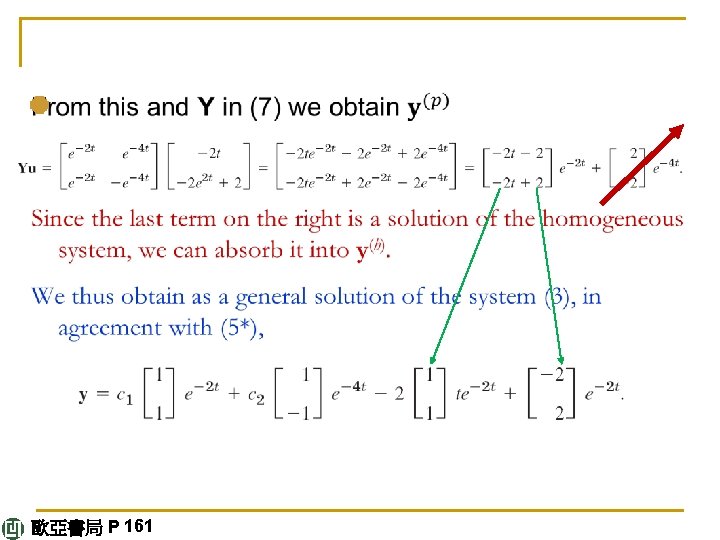
E X A M P L E 2 Solution by the Method of Variation of Parameters Solve (3) in Example 1. Solution. A basis of solutions of the homogeneous system is [e-2 t]T and [e-4 t -e-4 t]T. Hence the general solution (4) of the homogenous system may be written (7) continued 歐亞書局 P 161

Here, Y(t) = [y(1) y(2)] is the fundamental matrix (see Sec. 4. 2). As in Sec. 2. 10 we replace the constant vector c by a variable vector u(t) to obtain a particular solution (7’) y(p) = Y(t)u(t). Substitution into (3) y' = Ay + g gives (8) Y'u + Yu' = AYu + g. Now since y(1) and y(2) are solutions of the homogeneous system, we have y(1)' = Ay(1), y(2)' = Ay(2), thus Y' = AY. continued 歐亞書局 P 161

Hence Y'u = AYu, so that (8) reduces to Yu' = g. The solution is u' = Y-1 g; here we use that the inverse Y-1 of Y (Sec. 4. 0) exists because the determinant of Y is the Wronskian W, which is not zero for a basis. continued 歐亞書局 P 161

7. 8 Inverse of a Matrix. Gauss–Jordan Elimination Formulas for Inverses THEOREM 2 Inverse of a Matrix by Determinants The inverse of a nonsingular n × n matrix A = [ajk] is given by (4) where Cjk is the cofactor of ajk in det A (see Sec. 7. 7). Section 7. 8 p 85 歐亞書局 P

We multiply this by g, obtaining Integration is done component-wise and gives (where +2 comes from the lower limit of integration). continued 歐亞書局 P 161

SUMMARY OF CHAPTER 4 Whereas single electric circuits or single mass–spring systems are modeled by single ODEs (Chap. 2), networks of several circuits, systems of several masses and springs, and other engineering problems lead to systems of ODEs, involving several unknown functions y 1(t), ‥‥, yn(t). Of central interest are firstorder systems (Sec. 4. 2): y' = f(t, y), in components, continued 歐亞書局 P 164

to which higher order ODEs and systems of ODEs can be reduced (Sec. 4. 1). In this summary we let n = 2, so that y'1 = f 1(t, y 1, y 2) (1) y' = f(t, y), in components, y'2 = f 2(t, y 1, y 2) continued 歐亞書局 P 164

Then we can represent solution curves as trajectories in the phase plane (the y 1 y 2 -plane), investigate their totality [the “phase portrait” of (1)], and study the kind and stability of the critical points (points at which both ƒ 1 and ƒ 2 are zero), and classify them as nodes, saddle points, centers, or spiral points (Secs. 4. 3, 4. 4). These phase plane methods are qualitative; with their use we can discover various general properties of solutions without actually solving the system. They are primarily used for autonomous systems, that is, systems in which t does not occur explicitly. continued 歐亞書局 P 164

A linear system is of the form (2) If g = 0, the system is called homogeneous and is of the form (3) y' = Ay. continued 歐亞書局 P 164

If a 11, ‥‥, a 22 are constants, it has solutions y = xeλt, where λ is a solution of the quadratic equation and x ≠ 0 has components x 1, x 2 determined up to a multiplicative constant by (a 11 – λ)x 1 + a 12 x 2 = 0. (These λ’s are called the eigenvalues and these vectors x eigenvectors of the matrix A. Further explanation is given in Sec. 4. 0. ) continued 歐亞書局 P 165

A system (2) with g ≠ 0 is called nonhomogeneous. Its general solution is of the form y = yh + yp, where yh is a general solution of (3) and yp a particular solution of (2). Methods of determining the latter are discussed in Sec. 4. 6. The discussion of critical points of linear systems based on eigenvalues is summarized in Tables 4. 1 and 4. 2 in Sec. 4. 4. It also applies to nonlinear systems if the latter are first linearized. The key theorem for this is Theorem 1 in Sec. 4. 5, which also includes three famous applications, namely the pendulum and van der Pol equations and the Lotka– Volterra predator–prey population model. 歐亞書局 P 165