Chapter 4 Supervised learning Multilayer Networks II Other

Chapter 4 Supervised learning: Multilayer Networks II

Other Feedforward Networks • Madaline – Multiple adalines (of a sort) as hidden nodes – Weight change follows minimum disturbance principle • Adaptive multi-layer networks – Dynamically change the network size (# of hidden nodes) • Prediction networks – BP nets for prediction – Recurrent nets • Networks of radial basis function (RBF) – e. g. , Gaussian function – Perform better than sigmoid function (e. g. , interpolation) in function approximation • Some other selected types of layered NN

Madaline • Architectures – Hidden layers of adaline nodes – Output nodes differ • Learning – Error driven, but not by gradient descent – Minimum disturbance: smaller change of weights is preferred, provided it can reduce the error • Three Madaline models – Different node functions – Different learning rules (MR I, II, and III) – MR I and II developed in 60’s, MR III much later (88)

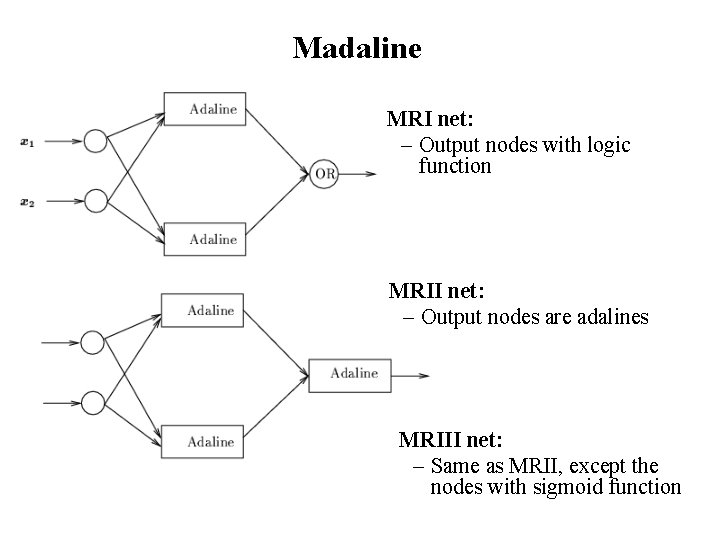
Madaline MRI net: – Output nodes with logic function MRII net: – Output nodes are adalines MRIII net: – Same as MRII, except the nodes with sigmoid function

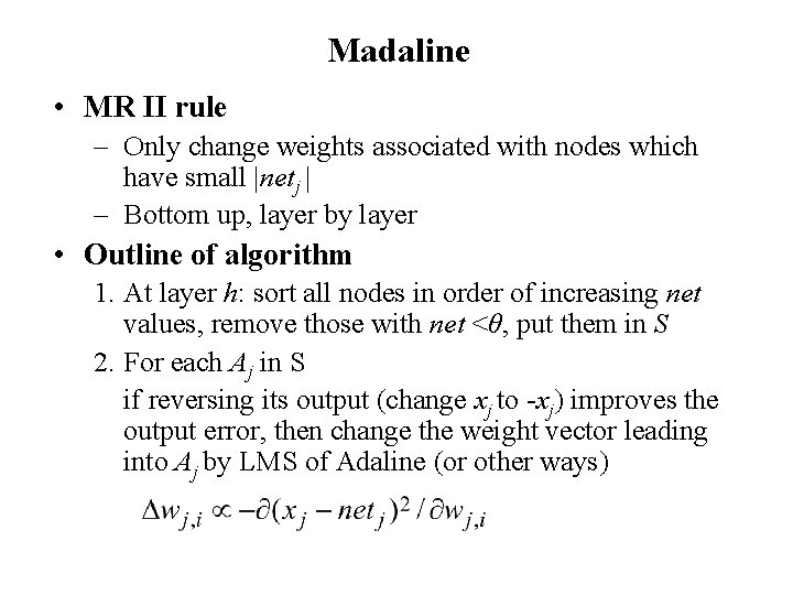
Madaline • MR II rule – Only change weights associated with nodes which have small |netj | – Bottom up, layer by layer • Outline of algorithm 1. At layer h: sort all nodes in order of increasing net values, remove those with net <θ, put them in S 2. For each Aj in S if reversing its output (change xj to -xj) improves the output error, then change the weight vector leading into Aj by LMS of Adaline (or other ways)

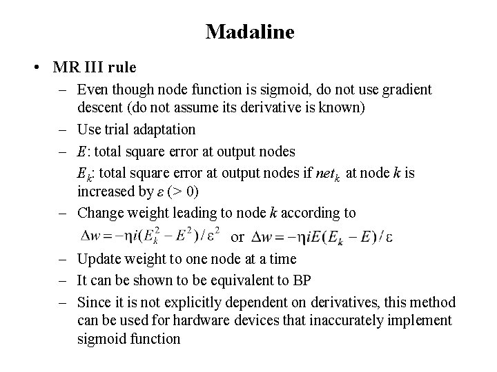
Madaline • MR III rule – Even though node function is sigmoid, do not use gradient descent (do not assume its derivative is known) – Use trial adaptation – E: total square error at output nodes Ek: total square error at output nodes if netk at node k is increased by ε (> 0) – Change weight leading to node k according to or – Update weight to one node at a time – It can be shown to be equivalent to BP – Since it is not explicitly dependent on derivatives, this method can be used for hardware devices that inaccurately implement sigmoid function

Adaptive Multilayer Networks • Smaller nets are often preferred – Computing is faster – Generalize better – Training is faster • Fewer weights to be trained • Smaller # of training samples needed • Heuristics for “optimal” net size – Pruning: start with a large net, then prune it by removing unimportant nodes and associated connections/weights – Growing: start with a very small net, then continuously increase its size with small increments until the performance becomes satisfactory – Combining the above two: a cycle of pruning and growing until performance is satisfied and no more pruning is possible

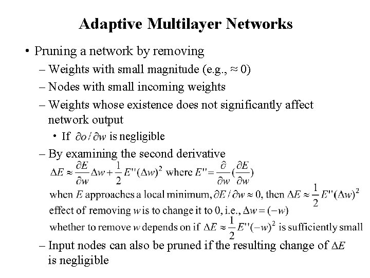
Adaptive Multilayer Networks • Pruning a network by removing – Weights with small magnitude (e. g. , ≈ 0) – Nodes with small incoming weights – Weights whose existence does not significantly affect network output • If is negligible – By examining the second derivative – Input nodes can also be pruned if the resulting change of is negligible

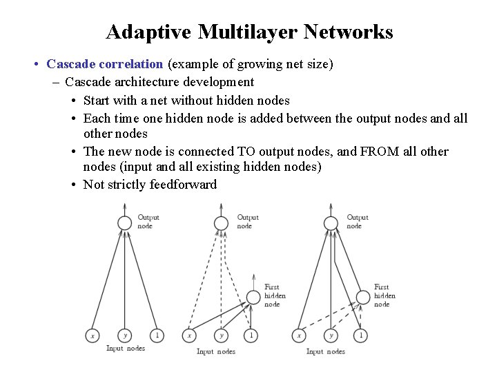
Adaptive Multilayer Networks • Cascade correlation (example of growing net size) – Cascade architecture development • Start with a net without hidden nodes • Each time one hidden node is added between the output nodes and all other nodes • The new node is connected TO output nodes, and FROM all other nodes (input and all existing hidden nodes) • Not strictly feedforward

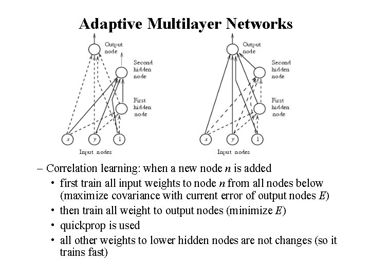
Adaptive Multilayer Networks – Correlation learning: when a new node n is added • first train all input weights to node n from all nodes below (maximize covariance with current error of output nodes E) • then train all weight to output nodes (minimize E) • quickprop is used • all other weights to lower hidden nodes are not changes (so it trains fast)

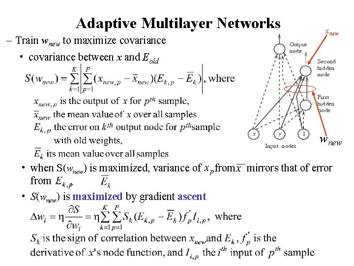
Adaptive Multilayer Networks – Train wnew to maximize covariance xnew • covariance between x and Eold wnew • when S(wnew) is maximized, variance of from mirrors that of error from , • S(wnew) is maximized by gradient ascent

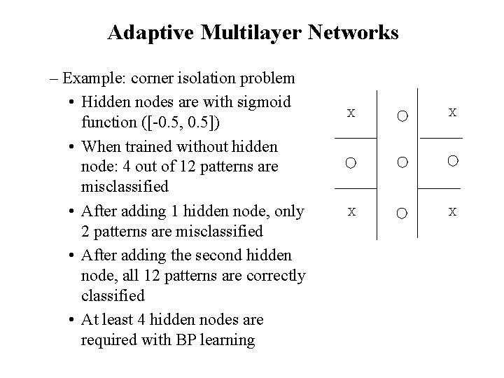
Adaptive Multilayer Networks – Example: corner isolation problem • Hidden nodes are with sigmoid function ([-0. 5, 0. 5]) • When trained without hidden node: 4 out of 12 patterns are misclassified • After adding 1 hidden node, only 2 patterns are misclassified • After adding the second hidden node, all 12 patterns are correctly classified • At least 4 hidden nodes are required with BP learning X X

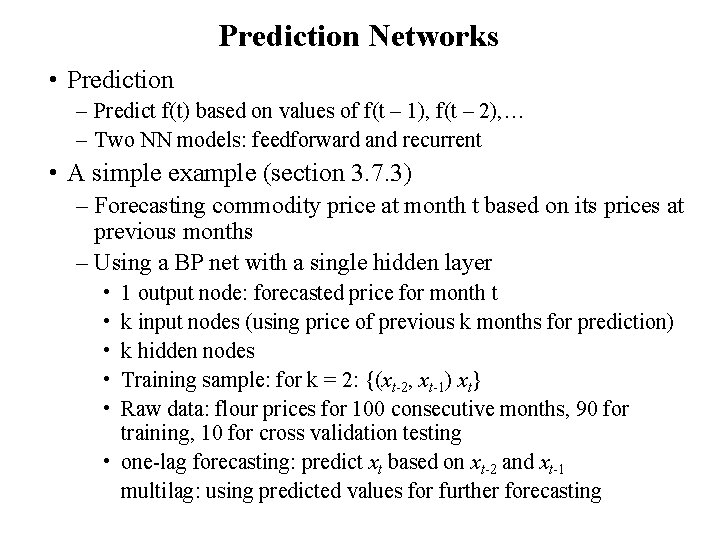
Prediction Networks • Prediction – Predict f(t) based on values of f(t – 1), f(t – 2), … – Two NN models: feedforward and recurrent • A simple example (section 3. 7. 3) – Forecasting commodity price at month t based on its prices at previous months – Using a BP net with a single hidden layer • • • 1 output node: forecasted price for month t k input nodes (using price of previous k months for prediction) k hidden nodes Training sample: for k = 2: {(xt-2, xt-1) xt} Raw data: flour prices for 100 consecutive months, 90 for training, 10 for cross validation testing • one-lag forecasting: predict xt based on xt-2 and xt-1 multilag: using predicted values for further forecasting

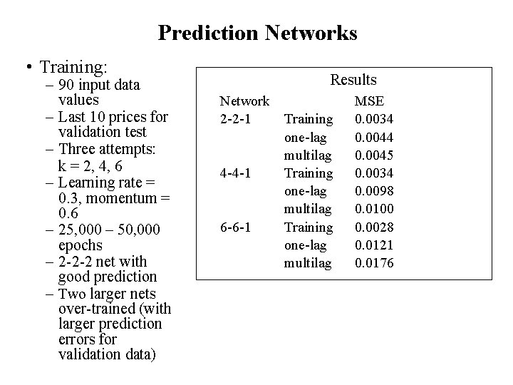
Prediction Networks • Training: – 90 input data values – Last 10 prices for validation test – Three attempts: k = 2, 4, 6 – Learning rate = 0. 3, momentum = 0. 6 – 25, 000 – 50, 000 epochs – 2 -2 -2 net with good prediction – Two larger nets over-trained (with larger prediction errors for validation data) Results Network 2 -2 -1 4 -4 -1 6 -6 -1 Training one-lag multilag MSE 0. 0034 0. 0045 0. 0034 0. 0098 0. 0100 0. 0028 0. 0121 0. 0176

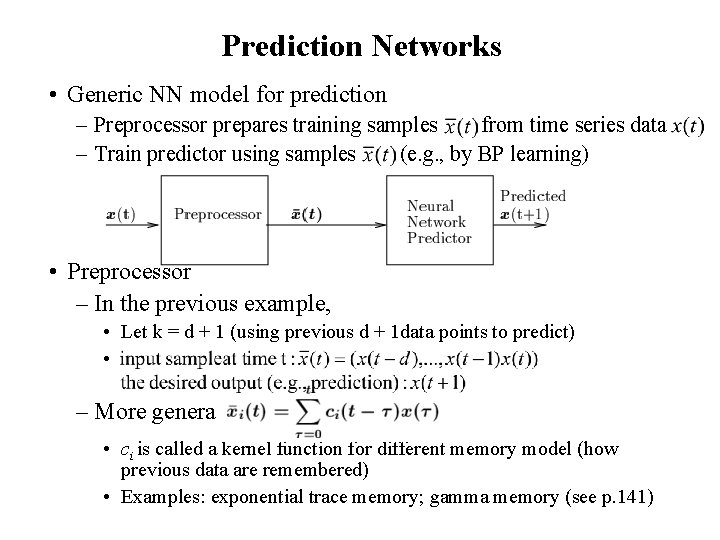
Prediction Networks • Generic NN model for prediction – Preprocessor prepares training samples from time series data – Train predictor using samples (e. g. , by BP learning) • Preprocessor – In the previous example, • Let k = d + 1 (using previous d + 1 data points to predict) • – More general: • ci is called a kernel function for different memory model (how previous data are remembered) • Examples: exponential trace memory; gamma memory (see p. 141)

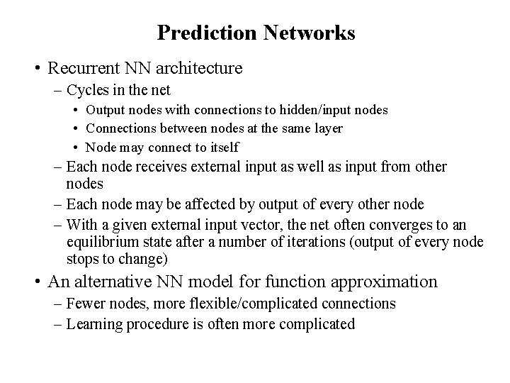
Prediction Networks • Recurrent NN architecture – Cycles in the net • Output nodes with connections to hidden/input nodes • Connections between nodes at the same layer • Node may connect to itself – Each node receives external input as well as input from other nodes – Each node may be affected by output of every other node – With a given external input vector, the net often converges to an equilibrium state after a number of iterations (output of every node stops to change) • An alternative NN model for function approximation – Fewer nodes, more flexible/complicated connections – Learning procedure is often more complicated

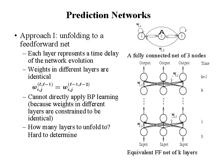
Prediction Networks • Approach I: unfolding to a feedforward net – Each layer represents a time delay of the network evolution – Weights in different layers are identical A fully connected net of 3 nodes – Cannot directly apply BP learning (because weights in different layers are constrained to be identical) – How many layers to unfold to? Hard to determine Equivalent FF net of k layers

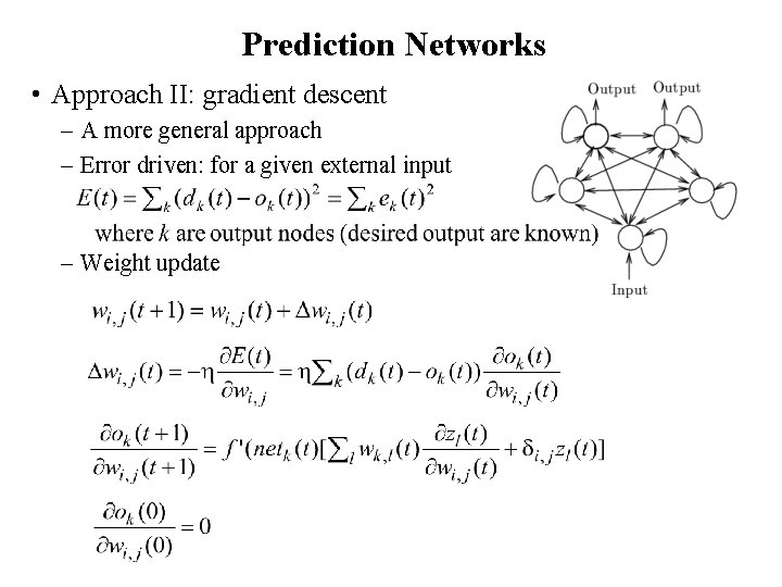
Prediction Networks • Approach II: gradient descent – A more general approach – Error driven: for a given external input – Weight update

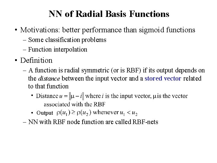
NN of Radial Basis Functions • Motivations: better performance than sigmoid functions – Some classification problems – Function interpolation • Definition – A function is radial symmetric (or is RBF) if its output depends on the distance between the input vector and a stored vector related to that function • • Output – NN with RBF node function are called RBF-nets

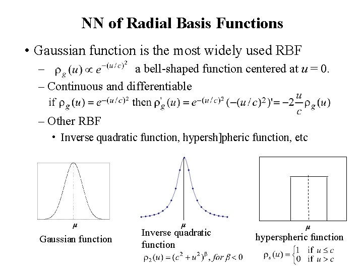
NN of Radial Basis Functions • Gaussian function is the most widely used RBF – a bell-shaped function centered at u = 0. – Continuous and differentiable – Other RBF • Inverse quadratic function, hypersh]pheric function, etc μ Gaussian function μ Inverse quadratic function μ hyperspheric function

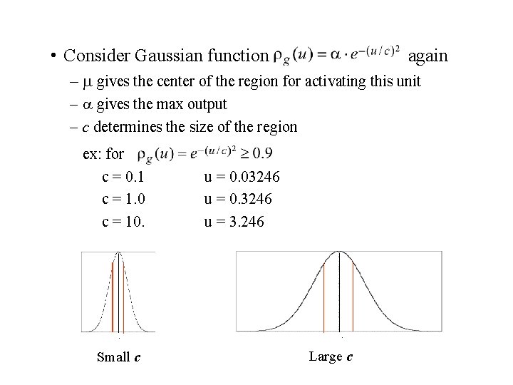
• Consider Gaussian function again – gives the center of the region for activating this unit – gives the max output – c determines the size of the region ex: for c = 0. 1 c = 1. 0 c = 10. Small c u = 0. 03246 u = 0. 3246 u = 3. 246 Large c

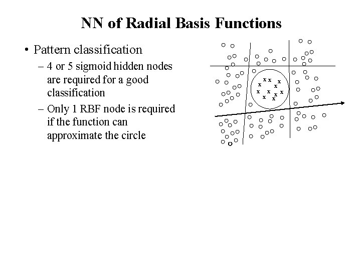
NN of Radial Basis Functions • Pattern classification – 4 or 5 sigmoid hidden nodes are required for a good classification – Only 1 RBF node is required if the function can approximate the circle x x x x xx

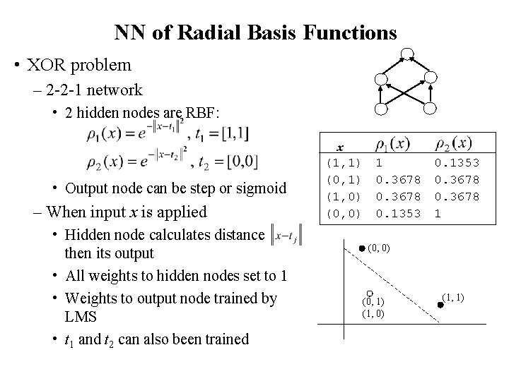
NN of Radial Basis Functions • XOR problem – 2 -2 -1 network • 2 hidden nodes are RBF: • Output node can be step or sigmoid – When input x is applied • Hidden node calculates distance then its output • All weights to hidden nodes set to 1 • Weights to output node trained by LMS • t 1 and t 2 can also been trained x (1, 1) (0, 1) (1, 0) (0, 0) 1 0. 3678 0. 1353 0. 3678 1 (0, 0) (0, 1) (1, 0) (1, 1)

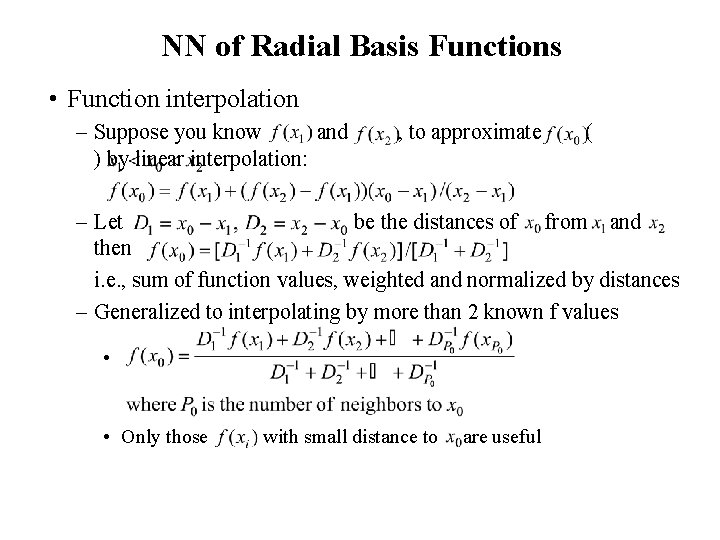
NN of Radial Basis Functions • Function interpolation – Suppose you know and ) by linear interpolation: , to approximate ( – Let be the distances of from and then i. e. , sum of function values, weighted and normalized by distances – Generalized to interpolating by more than 2 known f values • • Only those with small distance to are useful

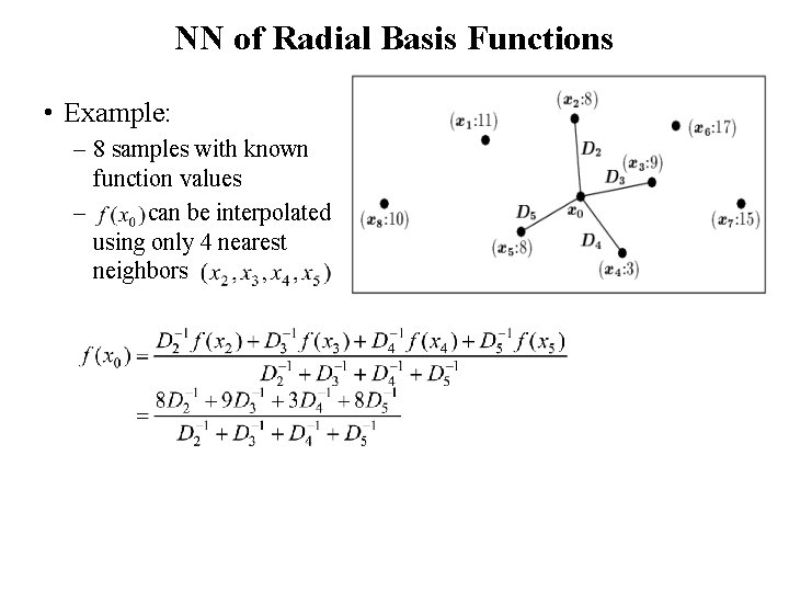
NN of Radial Basis Functions • Example: – 8 samples with known function values – can be interpolated using only 4 nearest neighbors

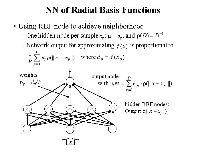
NN of Radial Basis Functions • Using RBF node to achieve neighborhood – One hidden node per sample xp: = xp, and – Network output for approximating weights wp = dp/P is proportional to output node hidden RBF nodes: Output (||x – xp||) x

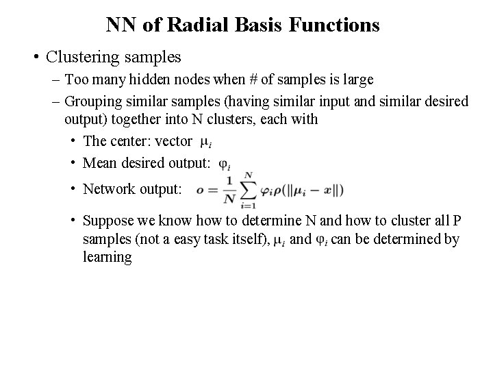
NN of Radial Basis Functions • Clustering samples – Too many hidden nodes when # of samples is large – Grouping similar samples (having similar input and similar desired output) together into N clusters, each with • The center: vector • Mean desired output: • Network output: • Suppose we know how to determine N and how to cluster all P samples (not a easy task itself), and can be determined by learning

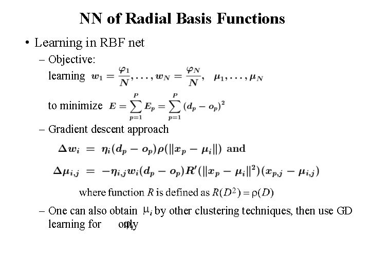
NN of Radial Basis Functions • Learning in RBF net – Objective: learning to minimize – Gradient descent approach – One can also obtain learning for only by other clustering techniques, then use GD

NN of Radial Basis Functions • A strategy for learning RBF net – Start with a single RBF hidden node for a single cluster containing only the first training sample. – For each of the new training samples x • If it is close to any of the existing clusters, do the gradient descent based updates of the w and φ for all clusters/hidden nodes • Otherwise, adding a new hidden node for a cluster containing only x • RBF networks are universal approximators – same representational power as BP networks

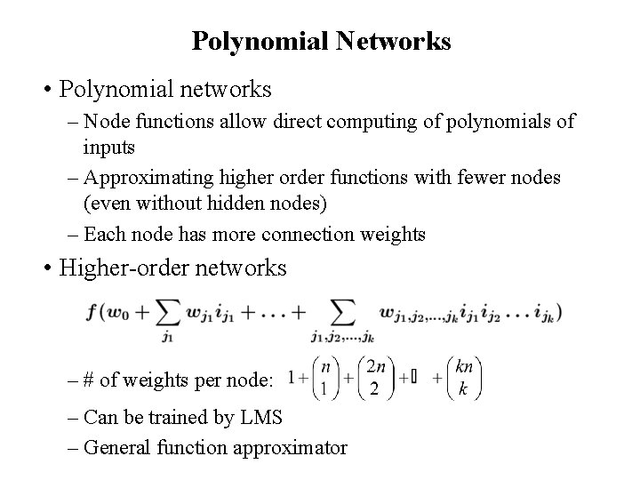
Polynomial Networks • Polynomial networks – Node functions allow direct computing of polynomials of inputs – Approximating higher order functions with fewer nodes (even without hidden nodes) – Each node has more connection weights • Higher-order networks – # of weights per node: – Can be trained by LMS – General function approximator

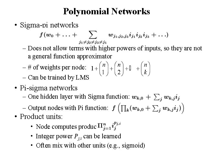
Polynomial Networks • Sigma-pi networks – Does not allow terms with higher powers of inputs, so they are not a general function approximator – # of weights per node: – Can be trained by LMS • Pi-sigma networks – One hidden layer with Sigma function: – Output nodes with Pi function: • Product units: • Node computes product: • Integer power Pj, i can be learned • Often mix with other units (e. g. , sigmoid)