Chapter 4 Strong and Weak Policy Effects in
- Slides: 26

Chapter 4 • Strong and Weak Policy Effects in the IS-LM Model Copyright © 2012 Pearson Addison-Wesley. All rights reserved.

The Definition of Money • Money is defined as any good or asset that serves the following three functions: – Medium of Exchange – Store of Value – Unit of Account • The Money Supply (MS) is equal to currency in circulation plus checking accounts at banks and thrift institutions. – The Fed is assumed to determine the money supply (see Chapter 13 for more details) Copyright © 2012 Pearson Addison-Wesley. All rights reserved. 4 -2

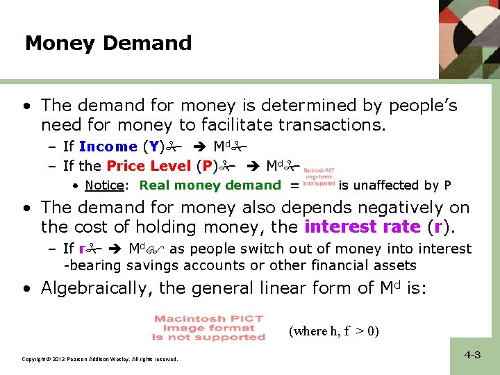
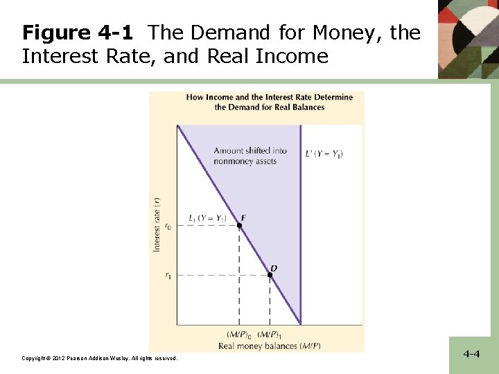
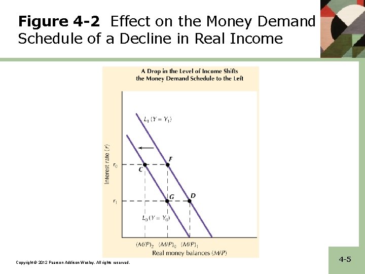
Money Demand • The demand for money is determined by people’s need for money to facilitate transactions. – If Income (Y) Md – If the Price Level (P) Md • Notice: Real money demand = is unaffected by P • The demand for money also depends negatively on the cost of holding money, the interest rate (r). – If r Md as people switch out of money into interest -bearing savings accounts or other financial assets • Algebraically, the general linear form of Md is: (where h, f > 0) Copyright © 2012 Pearson Addison-Wesley. All rights reserved. 4 -3

Figure 4 -1 The Demand for Money, the Interest Rate, and Real Income Copyright © 2012 Pearson Addison-Wesley. All rights reserved. 4 -4

Figure 4 -2 Effect on the Money Demand Schedule of a Decline in Real Income Copyright © 2012 Pearson Addison-Wesley. All rights reserved. 4 -5

What Shifts Money Demand? • The main shift factor for real Md is income (Y). • Additional shift factors include: – Interest paid on money: If money pays more interest (which was not possible before 1978), Md rises – Wealth: If people become wealthier, some of the additional wealth may be held as money, so Md rises. – Expected future inflation: If people expect P to rise quickly in the future, they will try to hold as little money as possible. – Payment technologies: Any technological development that alters how people pay for goods and services, or the ease of switching between money and non-money assets can change Md • Examples: Credit Cards and ATM’s Copyright © 2012 Pearson Addison-Wesley. All rights reserved. 4 -6

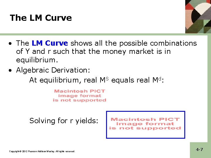
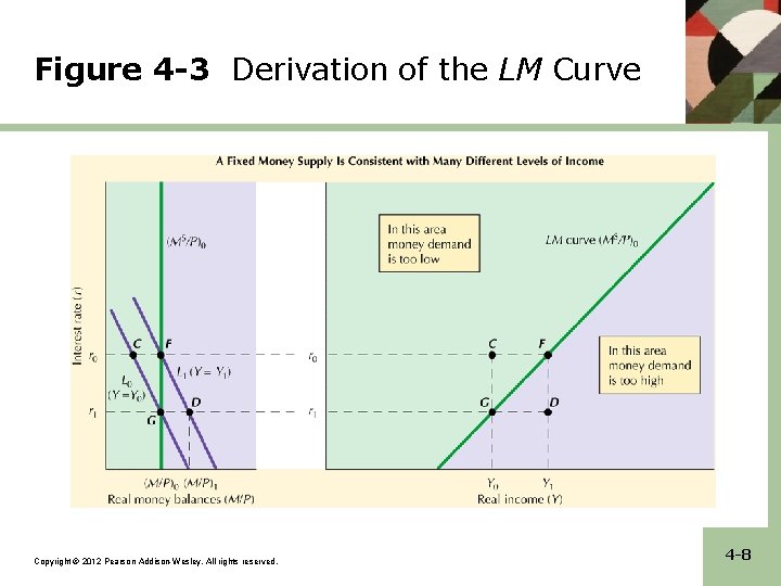
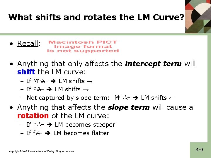
The LM Curve • The LM Curve shows all the possible combinations of Y and r such that the money market is in equilibrium. • Algebraic Derivation: At equilibrium, real MS equals real Md: Solving for r yields: Copyright © 2012 Pearson Addison-Wesley. All rights reserved. 4 -7

Figure 4 -3 Derivation of the LM Curve Copyright © 2012 Pearson Addison-Wesley. All rights reserved. 4 -8

What shifts and rotates the LM Curve? • Recall: • Anything that only affects the intercept term will shift the LM curve: – If MS LM shifts → – If P LM shifts → – Not captured by slope term: Md LM shifts ← • Anything that affects the slope term will cause a rotation of the LM curve: – If h LM becomes steeper – If f LM becomes flatter Copyright © 2012 Pearson Addison-Wesley. All rights reserved. 4 -9

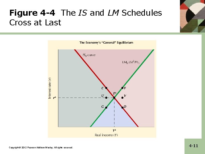
The General Equilibrium • A General Equilibrium is a situation of simultaneous equilibrium in all of the markets of the economy. • How does the economy adjust to the general equilibrium? – If the goods market is out of equilibrium involuntary inventory decumulation or accumulation occurs firms respond by increasing or decreasing production Y moves to equilibrium – If the money market is out of equilibrium pressure on interest rates will bring back monetary equilibrium Copyright © 2012 Pearson Addison-Wesley. All rights reserved. 4 -10

Figure 4 -4 The IS and LM Schedules Cross at Last Copyright © 2012 Pearson Addison-Wesley. All rights reserved. 4 -11

The IS/LM Model and the Global Economic Crisis • How can the Global Economic Crisis be modeled using the IS/LM model? • During the crisis, the IS curve shifted left. Why? – Household wealth and consumer optimism Cα – Business pessimism I – Greater difficulty in obtaining loans Cα and I • Summary: Private spending IS shifts Y , r Copyright © 2012 Pearson Addison-Wesley. All rights reserved. 4 -12

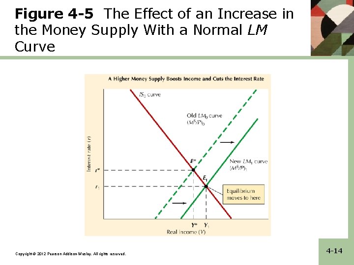
Monetary Policy • An expansionary monetary policy is one that has the effect of lowering interest rates and raising GDP • A contractionary monetary policy is one that has the effect of raising interest rates and lowering GDP Copyright © 2012 Pearson Addison-Wesley. All rights reserved. 4 -13

Figure 4 -5 The Effect of an Increase in the Money Supply With a Normal LM Curve Copyright © 2012 Pearson Addison-Wesley. All rights reserved. 4 -14

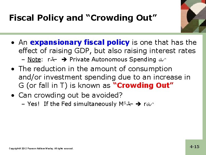
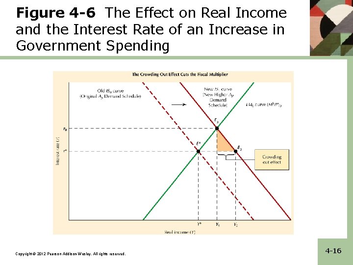
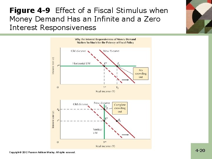
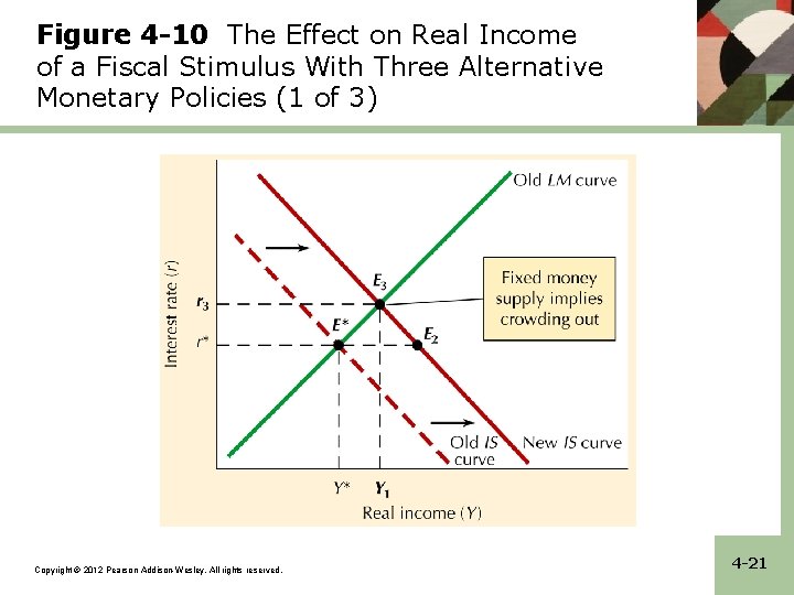
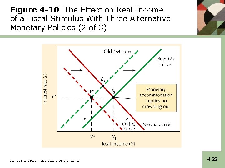
Fiscal Policy and “Crowding Out” • An expansionary fiscal policy is one that has the effect of raising GDP, but also raising interest rates – Note: r Private Autonomous Spending • The reduction in the amount of consumption and/or investment spending due to an increase in G (or fall in T) is known as “Crowding Out” • Can crowding out be avoided? – Yes! If the Fed simultaneously MS r Copyright © 2012 Pearson Addison-Wesley. All rights reserved. 4 -15

Figure 4 -6 The Effect on Real Income and the Interest Rate of an Increase in Government Spending Copyright © 2012 Pearson Addison-Wesley. All rights reserved. 4 -16

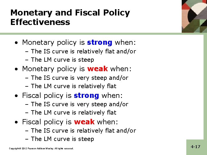
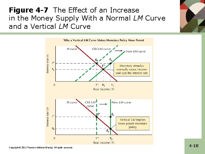
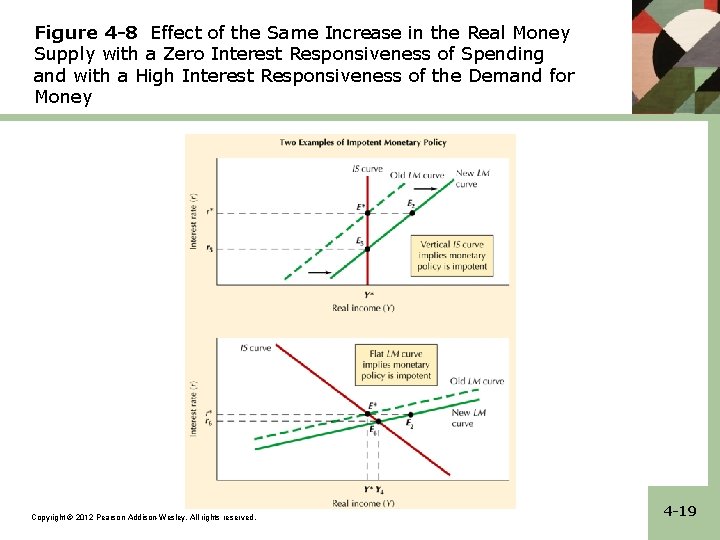
Monetary and Fiscal Policy Effectiveness • Monetary policy is strong when: – The IS curve is relatively flat and/or – The LM curve is steep • Monetary policy is weak when: – The IS curve is very steep and/or – The LM curve is relatively flat • Fiscal policy is strong when: – The IS curve is very steep and/or – The LM curve is relatively flat • Fiscal policy is weak when: – The IS curve is relatively flat and/or – The LM curve is steep Copyright © 2012 Pearson Addison-Wesley. All rights reserved. 4 -17

Figure 4 -7 The Effect of an Increase in the Money Supply With a Normal LM Curve and a Vertical LM Curve Copyright © 2012 Pearson Addison-Wesley. All rights reserved. 4 -18

Figure 4 -8 Effect of the Same Increase in the Real Money Supply with a Zero Interest Responsiveness of Spending and with a High Interest Responsiveness of the Demand for Money Copyright © 2012 Pearson Addison-Wesley. All rights reserved. 4 -19

Figure 4 -9 Effect of a Fiscal Stimulus when Money Demand Has an Infinite and a Zero Interest Responsiveness Copyright © 2012 Pearson Addison-Wesley. All rights reserved. 4 -20

Figure 4 -10 The Effect on Real Income of a Fiscal Stimulus With Three Alternative Monetary Policies (1 of 3) Copyright © 2012 Pearson Addison-Wesley. All rights reserved. 4 -21

Figure 4 -10 The Effect on Real Income of a Fiscal Stimulus With Three Alternative Monetary Policies (2 of 3) Copyright © 2012 Pearson Addison-Wesley. All rights reserved. 4 -22

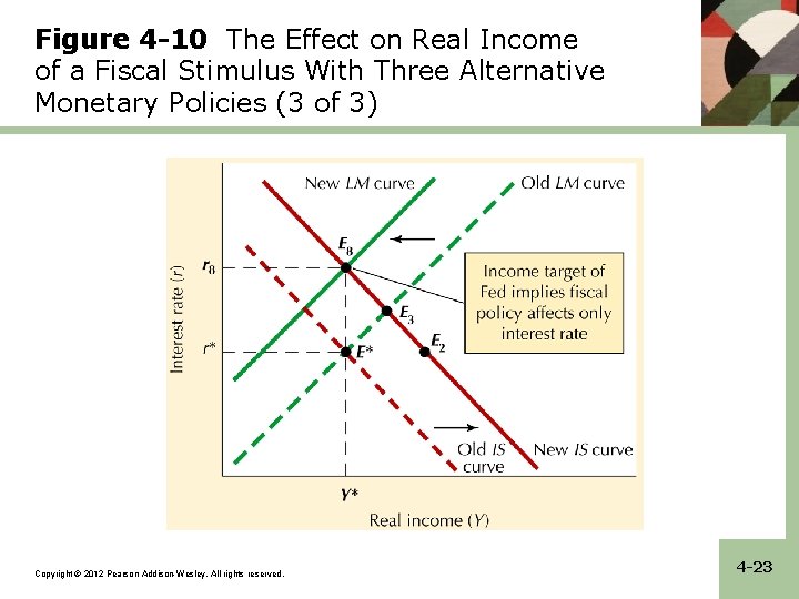
Figure 4 -10 The Effect on Real Income of a Fiscal Stimulus With Three Alternative Monetary Policies (3 of 3) Copyright © 2012 Pearson Addison-Wesley. All rights reserved. 4 -23

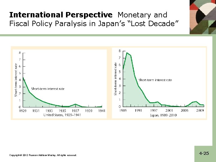
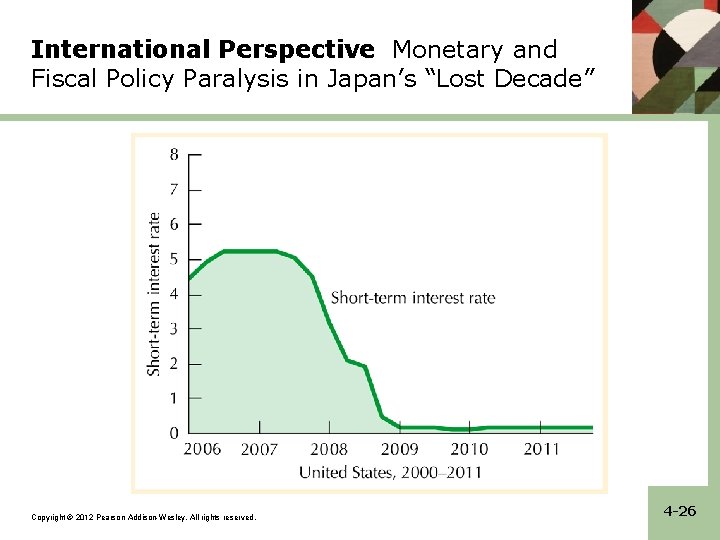
The Liquidity Trap • A Liquidity Trap occurs when investors are indifferent between holding money and short-term assets – Why might investors be indifferent? • Because the nominal interest rate on short-term assets is close to zero! – Why is a liquidity trap a problem? • Because the interest rate is close to zero, the Fed can no longer use monetary policy to lower the interest rate to boost output. • How is a liquidity trap represented? – The LM curve starts off horizontal at very low interest rates before having its normal upward slope Copyright © 2012 Pearson Addison-Wesley. All rights reserved. 4 -24

International Perspective Monetary and Fiscal Policy Paralysis in Japan’s “Lost Decade” Copyright © 2012 Pearson Addison-Wesley. All rights reserved. 4 -25

International Perspective Monetary and Fiscal Policy Paralysis in Japan’s “Lost Decade” Copyright © 2012 Pearson Addison-Wesley. All rights reserved. 4 -26