Chapter 4 Resources and Trade The HeckscherOhlin Model

Chapter 4 Resources and Trade: The Heckscher-Ohlin Model l l l Introduction A Model of a Two-Factor Economy Effects of International Trade Between Two-Factor Economies Empirical Evidence on the Heckscher-Ohlin Model Summary Appendix: Factor Prices, Goods Prices, and Input Choices 1

Introduction In the real world, while trade is partly explained by differences in labor productivity, it also reflects differences in countries’ resources. l The Heckscher-Ohlin theory: l – Emphasizes resource differences as the only source of trade – Shows that comparative advantage is influenced by: l l Relative factor abundance (refers to countries) Relative factor intensity (refers to goods) – Is also referred to as the factor-proportions theory 2

4 -1 A Model of a Two-Factor Economy § Assumptions of the Model • An economy can produce two goods, cloth and food. • The production of these goods requires two inputs • • that are in limited supply; labor (L) and land (T). Production of food is land-intensive and production of cloth is labor-intensive in both countries. Perfect competition prevails in all markets. 3

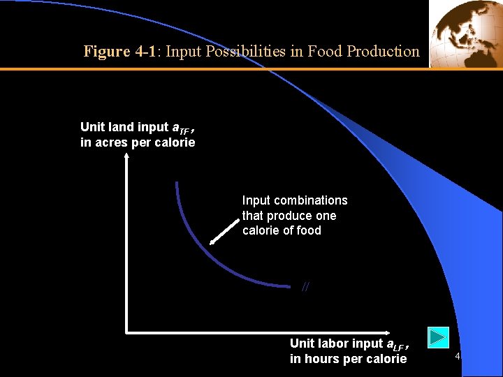
Figure 4 -1: Input Possibilities in Food Production Unit land input a. TF , in acres per calorie Input combinations that produce one calorie of food // Unit labor input a. LF , in hours per calorie 4

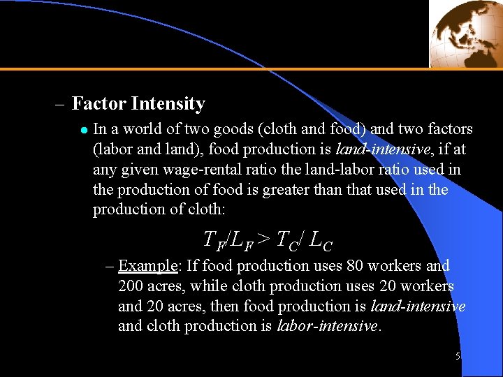
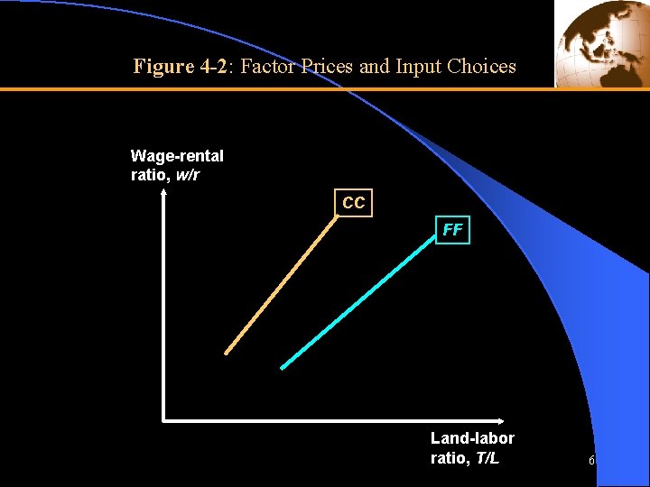
– Factor Intensity l In a world of two goods (cloth and food) and two factors (labor and land), food production is land-intensive, if at any given wage-rental ratio the land-labor ratio used in the production of food is greater than that used in the production of cloth: TF/LF > TC/ LC – Example: If food production uses 80 workers and 200 acres, while cloth production uses 20 workers and 20 acres, then food production is land-intensive and cloth production is labor-intensive. 5

Figure 4 -2: Factor Prices and Input Choices Wage-rental ratio, w/r CC FF Land-labor ratio, T/L 6

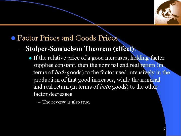
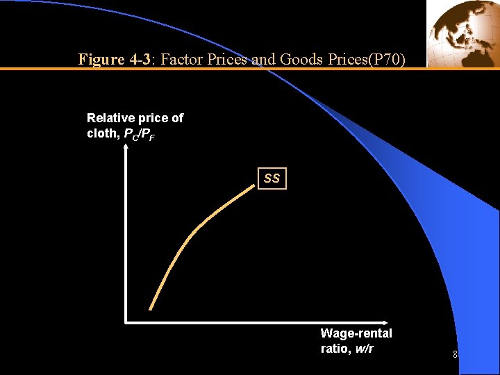
l Factor Prices and Goods Prices – Stolper-Samuelson Theorem (effect): l If the relative price of a good increases, holding factor supplies constant, then the nominal and real return (in terms of both goods) to the factor used intensively in the production of that good increases, while the nominal and real return (in terms of both goods) to the other factor decreases. – The reverse is also true. 7

Figure 4 -3: Factor Prices and Goods Prices(P 70) Relative price of cloth, PC/PF SS Wage-rental ratio, w/r 8

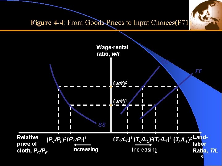
Figure 4 -4: From Goods Prices to Input Choices(P 71) Wage-rental ratio, w/r CC FF (w/r)2 (w/r)1 SS Relative (PC/PF)2 (PC/PF)1 price of Increasing cloth, PC/PF (TC/LC)1 (TC/LC)2(TF/LF)1 (TF/LF)2 Landlabor Increasing Ratio, T/L 9

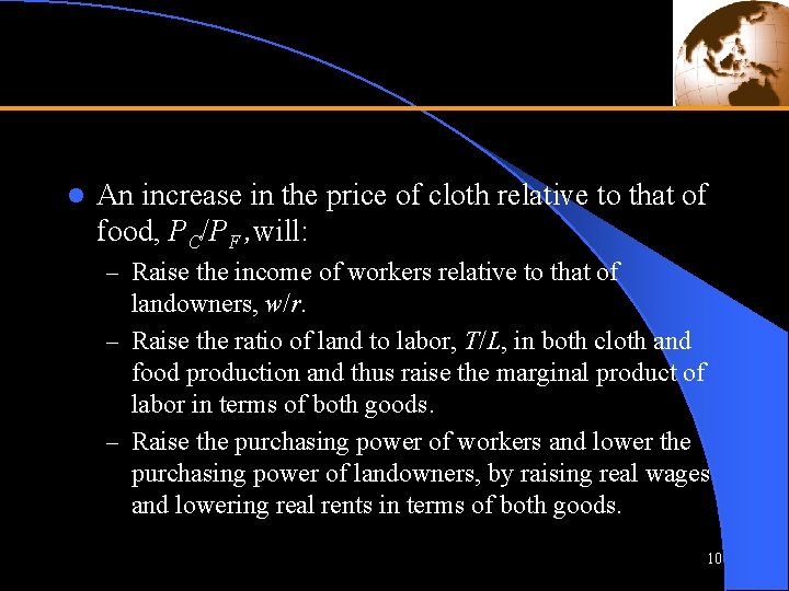
l An increase in the price of cloth relative to that of food, PC/PF , will: – Raise the income of workers relative to that of landowners, w/r. – Raise the ratio of land to labor, T/L, in both cloth and food production and thus raise the marginal product of labor in terms of both goods. – Raise the purchasing power of workers and lower the purchasing power of landowners, by raising real wages and lowering real rents in terms of both goods. 10

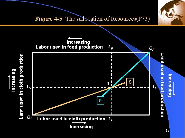
l Resources and Output – How is the allocation of resources determined? l Given the relative price of cloth and the supplies of land labor, it is possible to determine how much of each resource the economy devotes to the production of each good. 11

Figure 4 -5: The Allocation of Resources(P 73) 1 TC F OC Labor used in cloth production LC Increasing OF C TF Increasing Land used in cloth production LF Land used in food production Increasing Labor used in food production 12

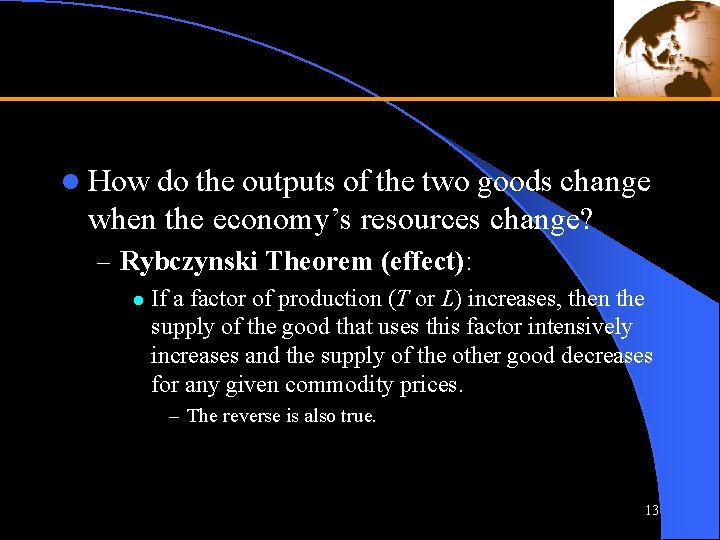
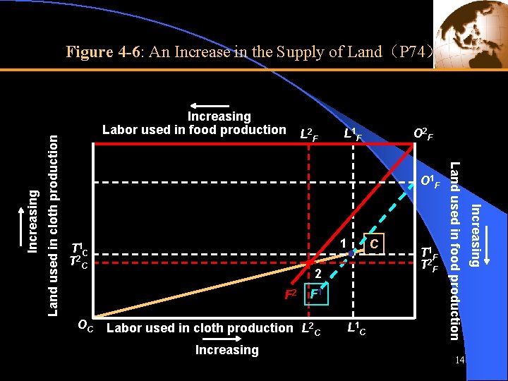
l How do the outputs of the two goods change when the economy’s resources change? – Rybczynski Theorem (effect): l If a factor of production (T or L) increases, then the supply of the good that uses this factor intensively increases and the supply of the other good decreases for any given commodity prices. – The reverse is also true. 13

L 2 F O 2 F L 1 F O 1 F 1 T 1 C T 2 C 2 F 2 OC C F 1 Labor used in cloth production L 2 C Increasing L 1 C T 1 F T 2 F 14 Increasing Land used in cloth production Increasing Labor used in food production Land used in food production Increasing Figure 4 -6: An Increase in the Supply of Land（P 74）

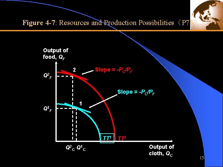
Figure 4 -7: Resources and Production Possibilities（P 75） Output of food, QF Q 2 F Slope = -PC/PF 2 Slope = -PC/PF Q 1 1 F TT 1 Q 2 C Q 1 C TT 2 Output of cloth, QC 15

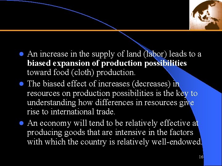
An increase in the supply of land (labor) leads to a biased expansion of production possibilities toward food (cloth) production. l The biased effect of increases (decreases) in resources on production possibilities is the key to understanding how differences in resources give rise to international trade. l An economy will tend to be relatively effective at producing goods that are intensive in the factors with which the country is relatively well-endowed. l 16

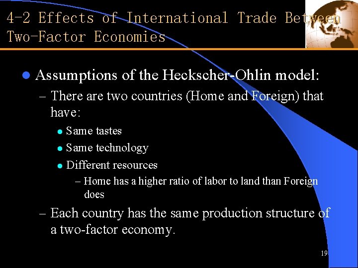
4 -2 Effects of International Trade Between Two-Factor Economies l Assumptions of the Heckscher-Ohlin model: – There are two countries (Home and Foreign) that have: Same tastes l Same technology l Different resources l – Home has a higher ratio of labor to land than Foreign does – Each country has the same production structure of a two-factor economy. 19

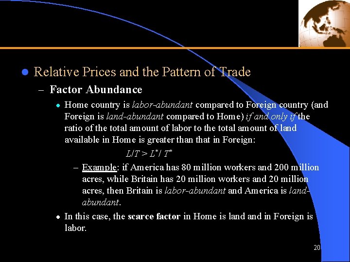
l Relative Prices and the Pattern of Trade – Factor Abundance l l Home country is labor-abundant compared to Foreign country (and Foreign is land-abundant compared to Home) if and only if the ratio of the total amount of labor to the total amount of land available in Home is greater than that in Foreign: L/T > L*/ T* – Example: if America has 80 million workers and 200 million acres, while Britain has 20 million workers and 20 million acres, then Britain is labor-abundant and America is landabundant. In this case, the scarce factor in Home is land in Foreign is labor. 20

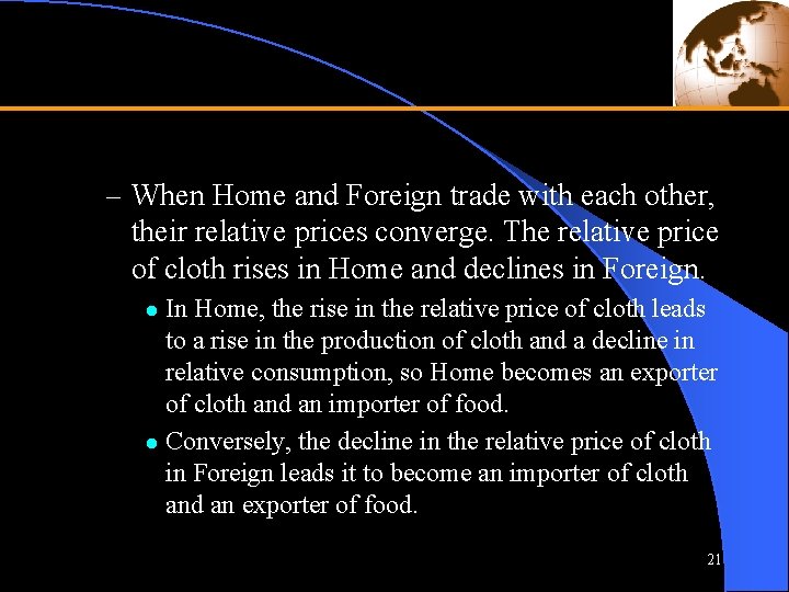
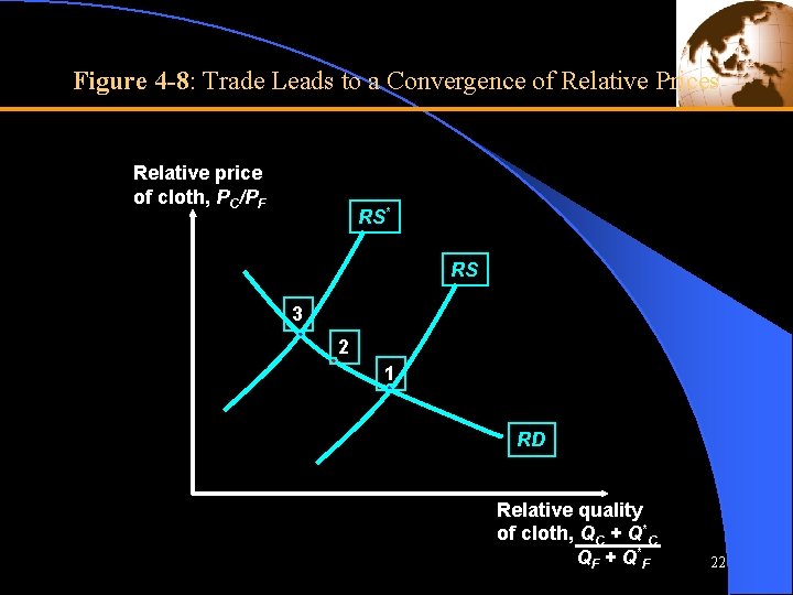
– When Home and Foreign trade with each other, their relative prices converge. The relative price of cloth rises in Home and declines in Foreign. In Home, the rise in the relative price of cloth leads to a rise in the production of cloth and a decline in relative consumption, so Home becomes an exporter of cloth and an importer of food. l Conversely, the decline in the relative price of cloth in Foreign leads it to become an importer of cloth and an exporter of food. l 21

Figure 4 -8: Trade Leads to a Convergence of Relative Prices Relative price of cloth, PC/PF RS* RS 3 2 1 RD Relative quality of cloth, QC + Q*C Q F + Q *F 22

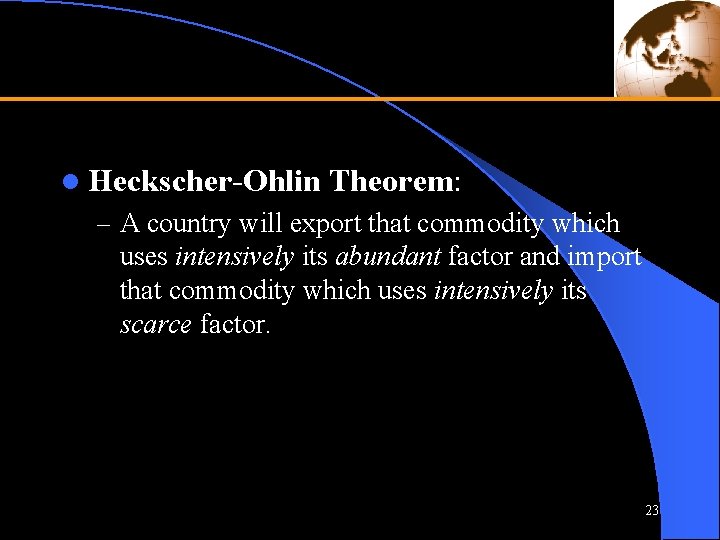
l Heckscher-Ohlin Theorem: – A country will export that commodity which uses intensively its abundant factor and import that commodity which uses intensively its scarce factor. 23

l Trade and the Distribution of Income – Trade produces a convergence of relative prices. – Changes in relative prices have strong effects on the relative earnings of labor and land in both countries: l In Home, where the relative price of cloth rises: – Laborers are made better off and landowners are made worse off. l In Foreign, where the relative price of cloth falls, the opposite happens: – Laborers are made worse off and landowners are made better off. – Owners of a country’s abundant factors gain from trade, but owners of a country’s scarce factors lose. 25

l Difference between the specific factors model and the Heckscher-Ohlin model in terms of income distribution effects: – The specificity of factors to particular industries is often only a temporary problem. l Example: Garment makers cannot become computer manufactures overnight, but given time the U. S. economy can shift its manufacturing employment from declining sectors to expanding ones. – In contrast, effects of trade on the distribution of income among land, labor, and capital are more or less permanent. 26

l Factor Price Equalization – In the absence of trade: labor would earn less in Home than in Foreign, and land would earn more. – Factor-Price Equalization Theorem: International trade leads to complete equalization in the relative and absolute returns to homogeneous factors across countries. l It implies that international trade is a substitute for the international mobility of factors. l 27

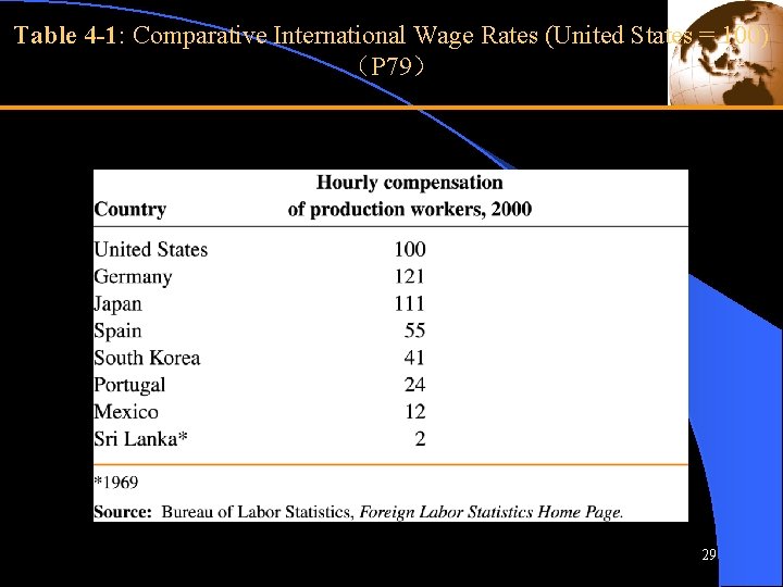
– Has international trade equalized the returns to homogeneous factors in different countries in the real world? l Even casual observation clearly indicates that it has not. – Example: Wages are much higher for doctors, engineers, technicians, mechanics and laborers in the United States and Germany than in Korea and Mexico. l Under these circumstances, it is more realistic to say that international trade has reduced, rather than completely eliminated, the international difference in the returns to homogeneous factors. 28

Table 4 -1: Comparative International Wage Rates (United States = 100) （P 79） 29

– Three assumptions crucial to the prediction of factor price equalization are in reality untrue: Both countries produce both goods l Both countries have the same technologies in production l Both countries have the same prices of goods due to trade l – One thing the factor-price equalization theorem does not say is that international trade will eliminate or reduce international differences in per capita incomes. 30

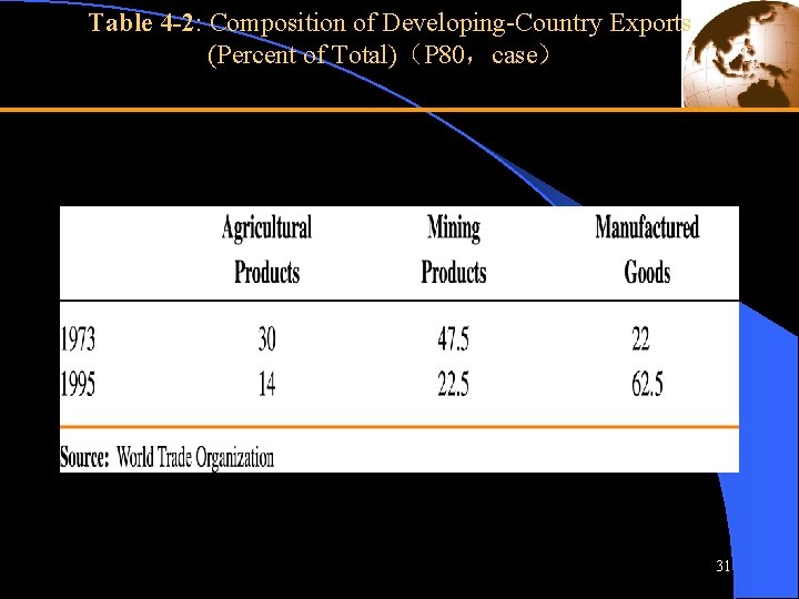
Table 4 -2: Composition of Developing-Country Exports (Percent of Total)（P 80，case） 31

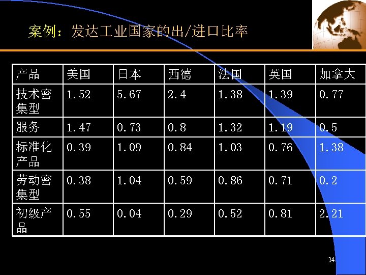
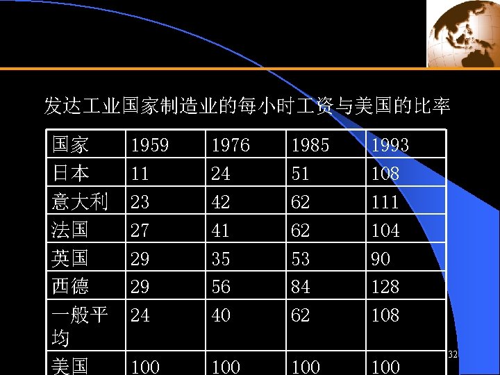
发达 业国家制造业的每小时 资与美国的比率 国家 日本 意大利 法国 英国 西德 一般平 均 美国 1959 11 23 27 29 29 24 100 1976 24 42 41 35 56 40 100 1985 51 62 62 53 84 62 100 1993 108 111 104 90 128 100 32

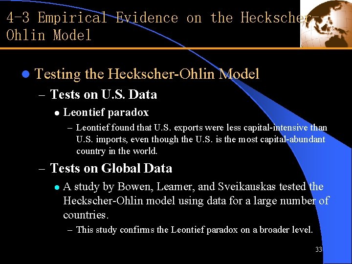
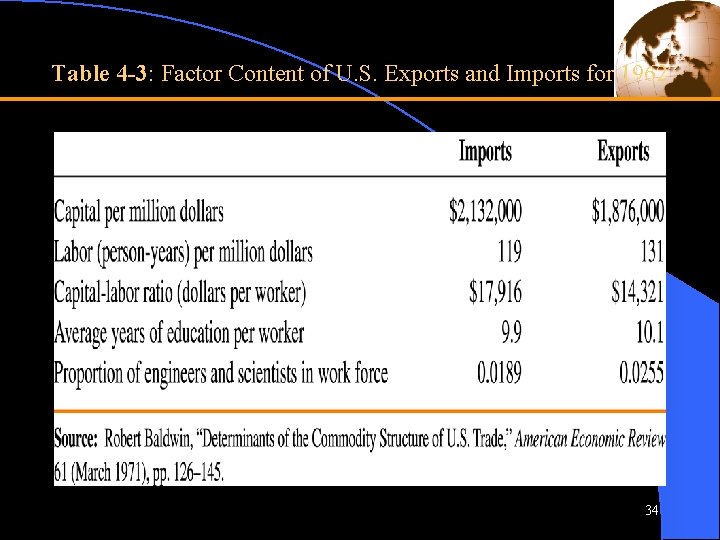
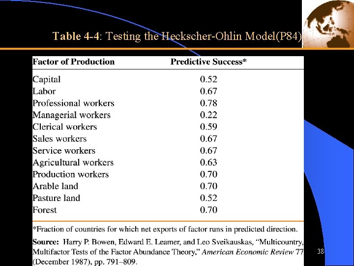
4 -3 Empirical Evidence on the Heckscher. Ohlin Model l Testing the Heckscher-Ohlin Model – Tests on U. S. Data l Leontief paradox – Leontief found that U. S. exports were less capital-intensive than U. S. imports, even though the U. S. is the most capital-abundant country in the world. – Tests on Global Data l A study by Bowen, Leamer, and Sveikauskas tested the Heckscher-Ohlin model using data for a large number of countries. – This study confirms the Leontief paradox on a broader level. 33

Table 4 -3: Factor Content of U. S. Exports and Imports for 1962 34

b、克拉维斯(Kravis)，1956年 C、基辛（Keesing)，1966年 d、鲍得温(Baldwin)，1971年 e、布朗逊(Branson)和莫挪尤斯(Monoyios)， 1977年 f、利默尔(Leamer)，1980，1984年 g、斯特思(Stern)和马斯库斯(Maskus)，1981年 h、萨尔瓦托(Salvatore)和巴拉扎什(Barazesh)： 1990年 36

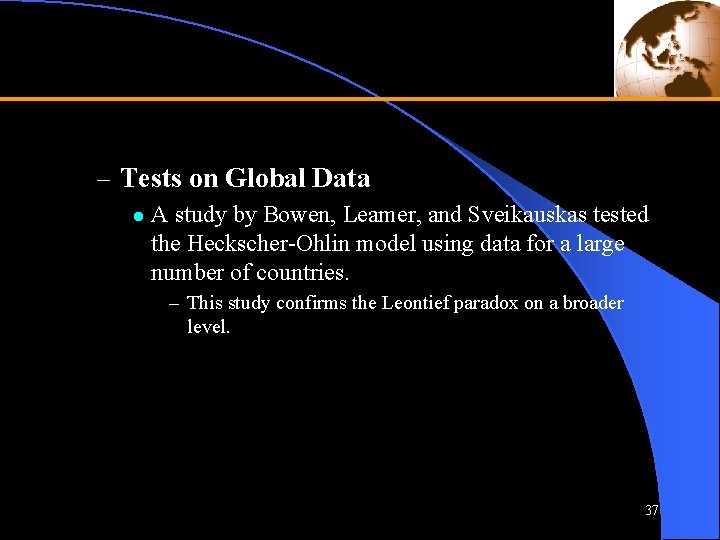
– Tests on Global Data l A study by Bowen, Leamer, and Sveikauskas tested the Heckscher-Ohlin model using data for a large number of countries. – This study confirms the Leontief paradox on a broader level. 37

Table 4 -4: Testing the Heckscher-Ohlin Model(P 84) 38

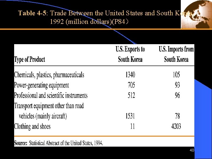
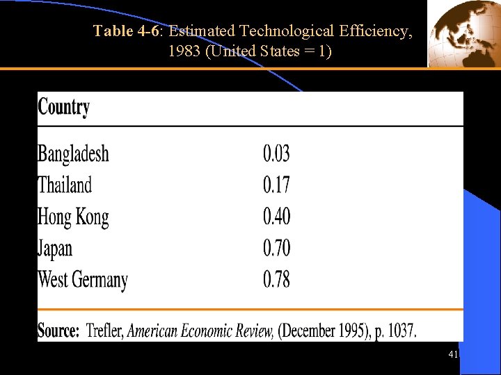
– Tests on North-South Trade l North-South trade in manufactures seems to fit the Heckscher-Ohlin theory much better than the overall pattern of international trade. – The Case of the Missing Trade l A study by Trefler in 1995 showed that technological differences across a sample of countries are very large. 39

Table 4 -5: Trade Between the United States and South Korea, 1992 (million dollars)(P 84） 40

Table 4 -6: Estimated Technological Efficiency, 1983 (United States = 1) 41

l Implications of the Tests – Empirical evidence on the Heckscher-Ohlin model has led to the following conclusions: It has been less successful at explaining the actual pattern of international trade. l It has been useful as a way to analyze the effects of trade on income distribution. l 42

Summary The Heckscher-Ohlin model, in which two goods are produced using two factors of production, emphasizes the role of resources in trade. l A rise in the relative price of the labor-intensive good will shift the distribution of income in favor of labor: l – The real wage of labor will rise in terms of both goods, while the real income of landowners will fall in terms of both goods. 43

Summary l For any given commodity prices, an increase in a factor of production increases the supply of the good that uses this factor intensively and reduces the supply of the other good. l The Heckscher-Ohlin theorem predicts the following pattern of trade: – A country will export that commodity which uses intensively its abundant factor and import that commodity which uses intensively its scarce factor. 44

Summary The owners of a country’s abundant factors gain from trade, but the owners of scarce factors lose. l In reality, complete factor price equalization is not observed because of wide differences in resources, barriers to trade, and international differences in technology. l Empirical evidence is mixed on the Heckscher. Ohlin model. l – Most researchers do not believe that differences in resources alone can explain the pattern of world trade or world factor prices. 45

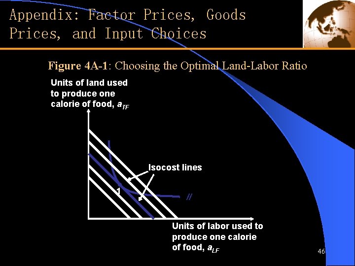
Appendix: Factor Prices, Goods Prices, and Input Choices Figure 4 A-1: Choosing the Optimal Land-Labor Ratio Units of land used to produce one calorie of food, a. TF Isocost lines 1 // Units of labor used to produce one calorie of food, a. LF 46

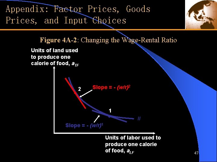
Appendix: Factor Prices, Goods Prices, and Input Choices Figure 4 A-2: Changing the Wage-Rental Ratio Units of land used to produce one calorie of food, a. TF 2 Slope = - (w/r)2 1 // Slope = - (w/r)1 Units of labor used to produce one calorie of food, a. LF 47

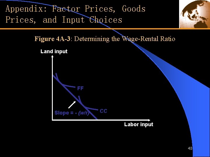
Appendix: Factor Prices, Goods Prices, and Input Choices Figure 4 A-3: Determining the Wage-Rental Ratio Land input FF Slope = - (w/r) CC Labor input 48

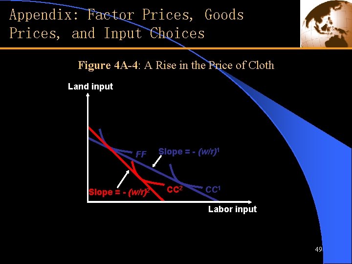
Appendix: Factor Prices, Goods Prices, and Input Choices Figure 4 A-4: A Rise in the Price of Cloth Land input FF Slope = - (w/r)2 Slope = - (w/r)1 CC 2 CC 1 Labor input 49