
Chapter 4 Relationships Between Categorical Variables Copyright 2011
Chapter 4 Relationships Between Categorical Variables Copyright © 2011 Brooks/Cole, Cengage Learning 1
Principle Question: Is there a relationship between the two variables, so that the category into which individuals fall for one variable seems to depend on the category they are in for the other variable? Copyright © 2011 Brooks/Cole, Cengage Learning 2
4. 1 Displaying Relationships Between Categorical Variables • Data displayed in a contingency or two-way table. • If one variable is explanatory, use it to define the rows of the table. • Two types of conditional percents: row percents and column percents. • Use row percents if the explanatory variable is the row variable. Copyright © 2011 Brooks/Cole, Cengage Learning 3
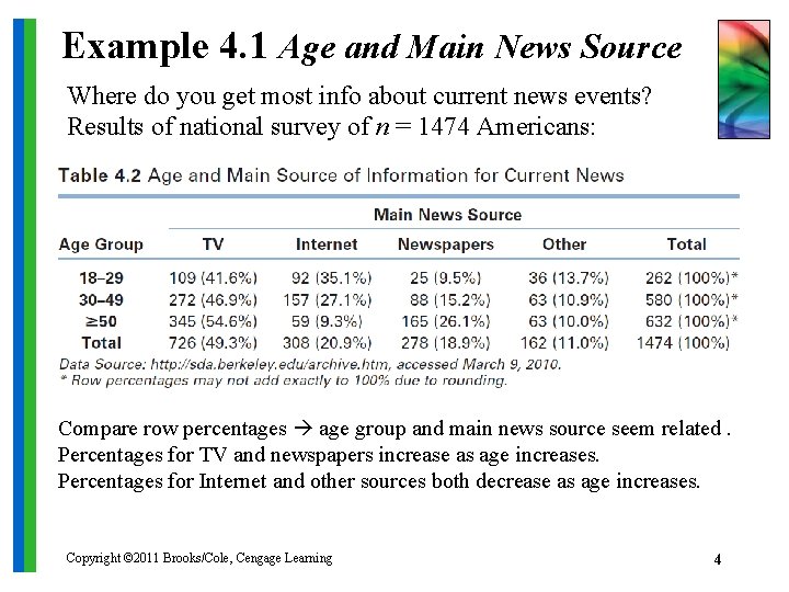
Example 4. 1 Age and Main News Source Where do you get most info about current news events? Results of national survey of n = 1474 Americans: Compare row percentages age group and main news source seem related. Percentages for TV and newspapers increase as age increases. Percentages for Internet and other sources both decrease as age increases. Copyright © 2011 Brooks/Cole, Cengage Learning 4
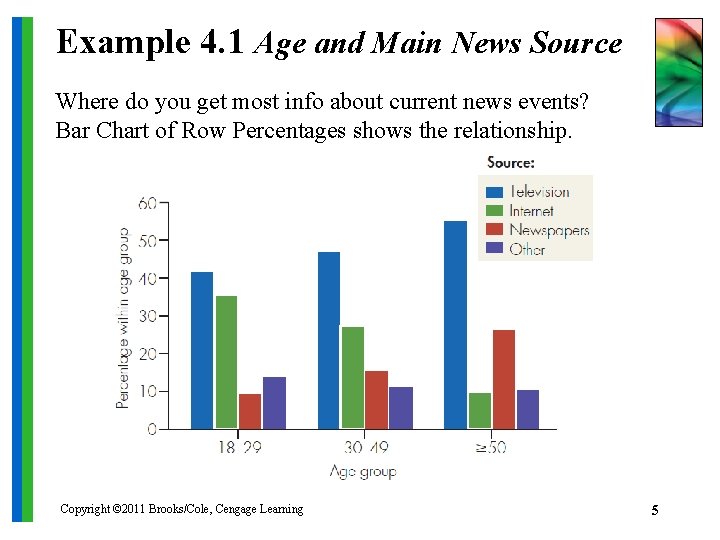
Example 4. 1 Age and Main News Source Where do you get most info about current news events? Bar Chart of Row Percentages shows the relationship. Copyright © 2011 Brooks/Cole, Cengage Learning 5
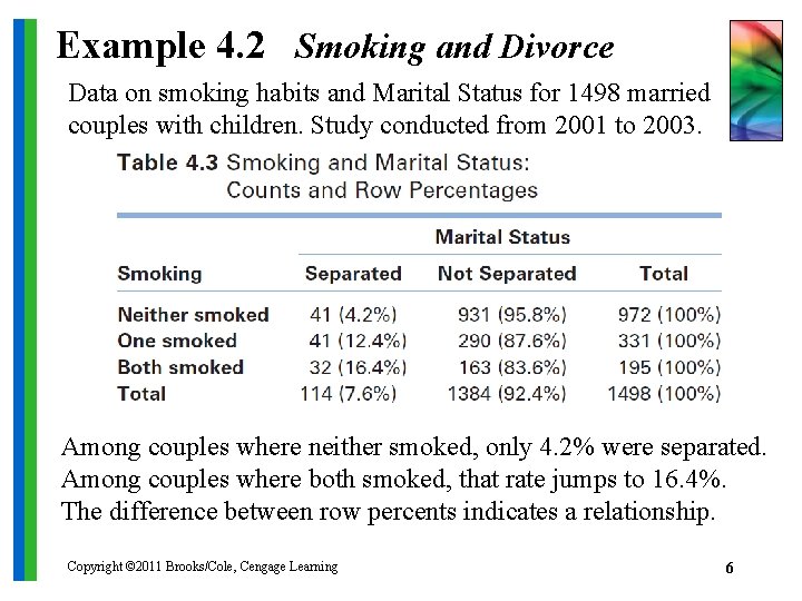
Example 4. 2 Smoking and Divorce Data on smoking habits and Marital Status for 1498 married couples with children. Study conducted from 2001 to 2003. Among couples where neither smoked, only 4. 2% were separated. Among couples where both smoked, that rate jumps to 16. 4%. The difference between row percents indicates a relationship. Copyright © 2011 Brooks/Cole, Cengage Learning 6
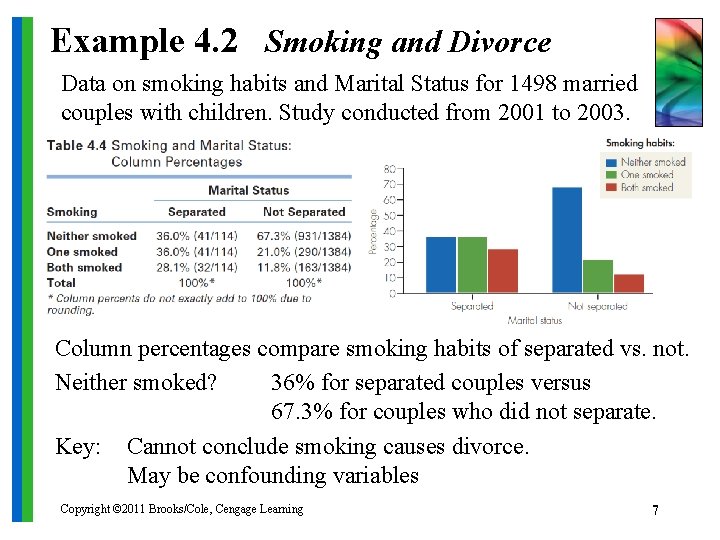
Example 4. 2 Smoking and Divorce Data on smoking habits and Marital Status for 1498 married couples with children. Study conducted from 2001 to 2003. Column percentages compare smoking habits of separated vs. not. Neither smoked? 36% for separated couples versus 67. 3% for couples who did not separate. Key: Cannot conclude smoking causes divorce. May be confounding variables Copyright © 2011 Brooks/Cole, Cengage Learning 7
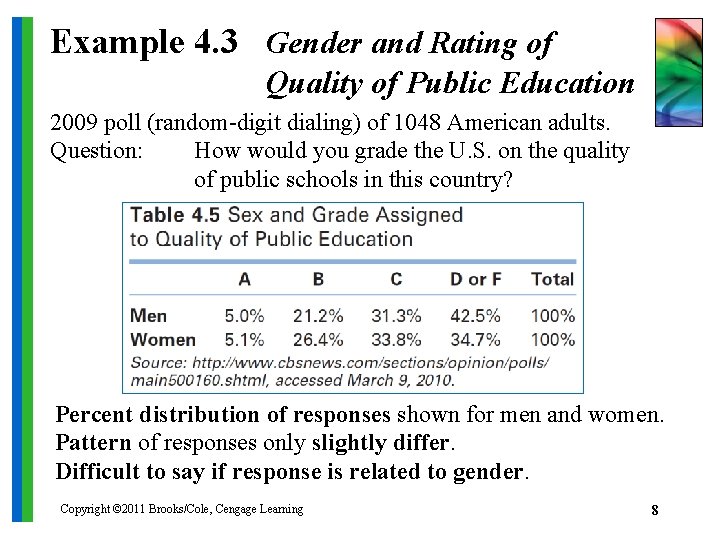
Example 4. 3 Gender and Rating of Quality of Public Education 2009 poll (random-digit dialing) of 1048 American adults. Question: How would you grade the U. S. on the quality of public schools in this country? Percent distribution of responses shown for men and women. Pattern of responses only slightly differ. Difficult to say if response is related to gender. Copyright © 2011 Brooks/Cole, Cengage Learning 8
4. 4 Assessing the Statistical Significance of a 2 x 2 Table Question: Can the relationship observed in the sample data be inferred to hold in the population represented by the data? A statistically significant relationship or difference is one that is large enough to be unlikely to have occurred in the observed sample if there is no relationship or difference in the population. Copyright © 2011 Brooks/Cole, Cengage Learning 9
Five Steps to Determining Statistical Significance: 1. Determine the null and alternative hypotheses. 2. Summarize the data into an appropriate test statistic after first verifying necessary data conditions met. 3. Find the p-value, the probability the test statistic would be as extreme as it is, or more so, calculated assuming the null hypothesis is true. 4. Decide whether or not the result is statistically significant based on the p-value. 5. Report the conclusion in the context of the situation. Copyright © 2011 Brooks/Cole, Cengage Learning 10
Step 1: Null and Alternative Hypotheses Null hypothesis: The two variables are not related in the population. Alternative hypothesis: The two variables are related in the population. Copyright © 2011 Brooks/Cole, Cengage Learning 11
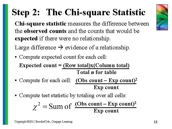
Step 2: The Chi-square Statistic Chi-square statistic measures the difference between the observed counts and the counts that would be expected if there were no relationship. Large difference evidence of a relationship. • Compute expected count for each cell: Expected count = (Row total)x(Column total) Total n for table • Compute for each cell: (Obs count – Exp count)2 Exp count • Compute test statistic by totaling over all cells: (Obs count – Exp count)2 Exp count Copyright © 2011 Brooks/Cole, Cengage Learning 12
Step 3: The p-value of the Chi-square Test Large test statistic evidence of a relationship. So how large is enough to declare significance? Q: If there is actually no relationship in the population, what is the likelihood that the chi-square statistic could be as large as it is or larger? A: The p-value Note: The p-value is generally reported in computer output. Copyright © 2011 Brooks/Cole, Cengage Learning 13
Steps 4 and 5: Making and Reporting a Decision Large test statistic small p-value evidence a real relationship exists in the population. Common rule: • p-value 0. 05 say relationship is statistically significant and we reject the null hypothesis • p-value > 0. 05 cannot say relationship is statistically significant and we cannot reject the null hypothesis Note: For 2 x 2 tables, a test statistic of 3. 84 or larger is significant. Copyright © 2011 Brooks/Cole, Cengage Learning 14
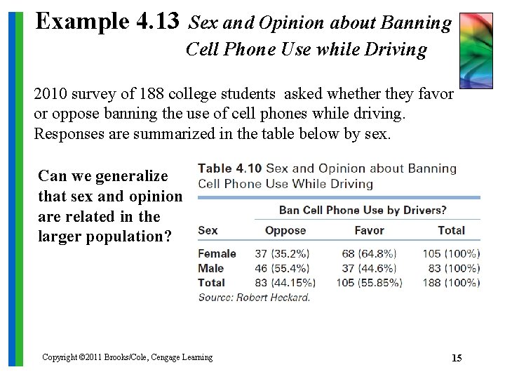
Example 4. 13 Sex and Opinion about Banning Cell Phone Use while Driving 2010 survey of 188 college students asked whether they favor or oppose banning the use of cell phones while driving. Responses are summarized in the table below by sex. Can we generalize that sex and opinion are related in the larger population? Copyright © 2011 Brooks/Cole, Cengage Learning 15
Example 4. 13 Sex and Opinion about Banning Cell Phone Use while Driving Null hypothesis: Sex and opinion about banning cell phone use by drivers are not related. Alternative hypothesis: Sex and opinion about banning cell phone use by drivers are related. Chi-squared test statistic is 7. 659. p-value is 0. 006 since the p-value is less than 0. 05, we can say that the relationship is statistically significant. We can reject the null hypothesis and infer that sex and opinion about banning cell phone use while driving are related in the population represented by these students. Copyright © 2011 Brooks/Cole, Cengage Learning 16
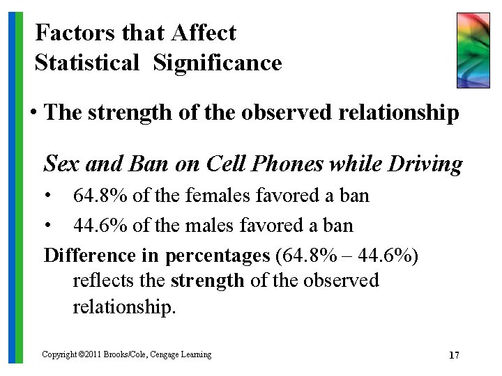
Factors that Affect Statistical Significance • The strength of the observed relationship Sex and Ban on Cell Phones while Driving • 64. 8% of the females favored a ban • 44. 6% of the males favored a ban Difference in percentages (64. 8% – 44. 6%) reflects the strength of the observed relationship. Copyright © 2011 Brooks/Cole, Cengage Learning 17

Factors that Affect Statistical Significance: (cont) • How many people were studied Example: I. Treatment A had 8 of 10 patients improve. Treatment B had 5 of 10 patients improve. Strength = 80% - 50% = 30% seems large but study is too small. The p-value is 0. 16. II. Treatment A had 80 of 100 patients improve. Treatment B had 50 of 100 patients improve. Strength = 80% - 50% = 30% is again large. The p-value is 0. 000000087, which is very significant. Copyright © 2011 Brooks/Cole, Cengage Learning 18
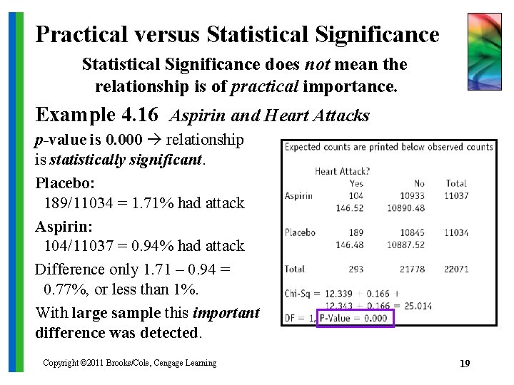
Practical versus Statistical Significance does not mean the relationship is of practical importance. Example 4. 16 Aspirin and Heart Attacks p-value is 0. 000 relationship is statistically significant. Placebo: 189/11034 = 1. 71% had attack Aspirin: 104/11037 = 0. 94% had attack Difference only 1. 71 – 0. 94 = 0. 77%, or less than 1%. With large sample this important difference was detected. Copyright © 2011 Brooks/Cole, Cengage Learning 19
Interpreting a Nonsignificant Result • The sample results are not strong enough to safely conclude that there is a relationship in the population. • The observed relationship in the sample could have resulted by chance, when in fact there is no relationship in the population. Copyright © 2011 Brooks/Cole, Cengage Learning 20
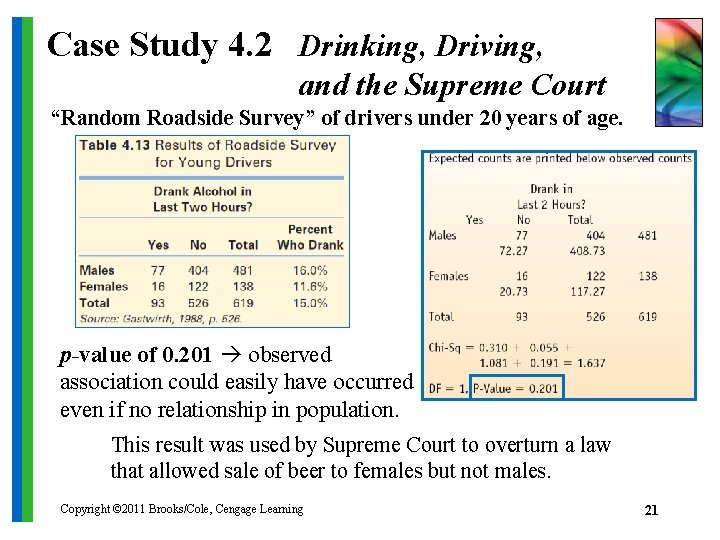
Case Study 4. 2 Drinking, Driving, and the Supreme Court “Random Roadside Survey” of drivers under 20 years of age. p-value of 0. 201 observed association could easily have occurred even if no relationship in population. This result was used by Supreme Court to overturn a law that allowed sale of beer to females but not males. Copyright © 2011 Brooks/Cole, Cengage Learning 21
- Slides: 21