Chapter 4 Reasoning with Constraints Textbook Artificial Intelligence

Chapter 4: Reasoning with Constraints Textbook: Artificial Intelligence Foundations of Computational Agents, 2 nd Edition, David L. Poole and Alan K Mackworth, Cambridge University Press, 2018. Asst. Prof. Dr. Anilkumar K. G 1

Introduction • States can be described in terms of features for reasoning – It is better to perform reasoning on these features. • Features are described using variables • In planning and scheduling, an agent assigns a time for each action • These assignments must satisfy certain constraints in the order of actions that can be carried out towards a goal – The problems dealing with constrains to achieve a goal is called constraint satisfaction problems Asst. Prof. Dr. Anilkumar K. G 2

Variables and Worlds • Constraint satisfaction problems are described in terms of their variables and possible worlds – A possible world is a possible way the world (the real world or some imaginary world) could be • For example, when representing a crossword puzzle, the possible worlds correspond to the ways the crossword could be filled out. • Possible worlds are described by algebraic variables – An algebraic variable is a symbol used to denote features of possible worlds. – Algebraic variables are written starting with an upper-case letter. – Each algebraic variable X has an associated domain, indicated as dom(X), which is the set of values the variable can take – Asst. Prof. Dr. Anilkumar K. G 3

Variables and Worlds • A discrete variable is one whose domain is finite or countable • A binary variable is a discrete variable with two values in its domain. – A binary variable is a Boolean variable, with domain {true, false}. • We can also have variables that are not discrete; – for example, a variable whose domain corresponds to a real line or an interval is a continuous variable. Asst. Prof. Dr. Anilkumar K. G 4

Variables and Worlds • Given a set of variables, an assignment on the set of variables is a function from the variables into the domains of the variables – an assignment on {X 1, X 2, . . , Xk} as {X 1 = v 1, X 2 = v 2, . . , Xk = vk}, where vi is in dom(Xi). – This assignment specifies that, for each i, variable Xi is assigned value vi. • A total assignment assigns all of the variables – A possible world is defined to be a total assignment • It is a function from variables into values that assigns a value to every variable. Asst. Prof. Dr. Anilkumar K. G 5

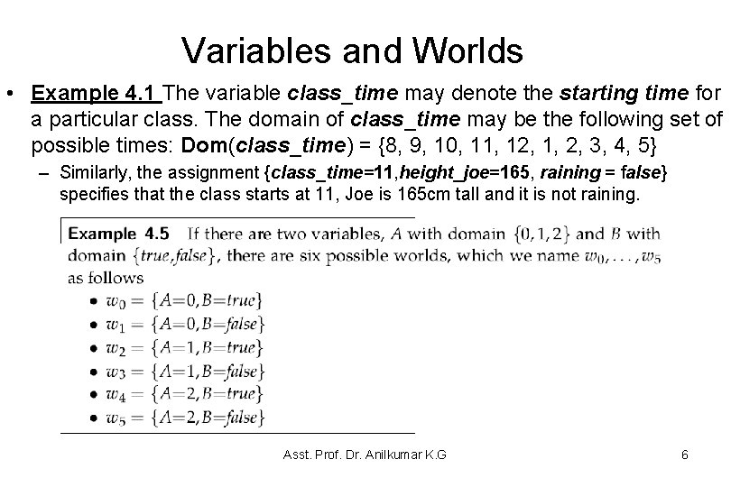
Variables and Worlds • Example 4. 1 The variable class_time may denote the starting time for a particular class. The domain of class_time may be the following set of possible times: Dom(class_time) = {8, 9, 10, 11, 12, 1, 2, 3, 4, 5} – Similarly, the assignment {class_time=11, height_joe=165, raining = false} specifies that the class starts at 11, Joe is 165 cm tall and it is not raining. Asst. Prof. Dr. Anilkumar K. G 6

Variables and Worlds • If there are n variables, each with domain size d, there are dn possible worlds – 10 binary variables can describe 1, 024 (210) worlds – 20 binary variables can describe 1, 048, 576 (220)worlds • One main advantage of reasoning in terms of variables is the computational savings – Reasoning in terms of thirty variables may be easier than reasoning in terms of more than a billion worlds. – Many real-world problems have thousands of variables Asst. Prof. Dr. Anilkumar K. G 7

Constraints • In many domains, not all possible assignments to variables are permissible – A hard constraint, or constraint, specifies legal combinations of assignments of values to some of the variables • A scope is a set of variables in a domain – A relation on a scope S is a function from assignments on S to {true, false} • it specifies whether each assignment is true or false – A constraint is said to involve each of the variables in its scope • A possible world w satisfies a set of constraints if, for every constraint, the values assigned in w to the variables satisfies the constraint. Asst. Prof. Dr. Anilkumar K. G 8

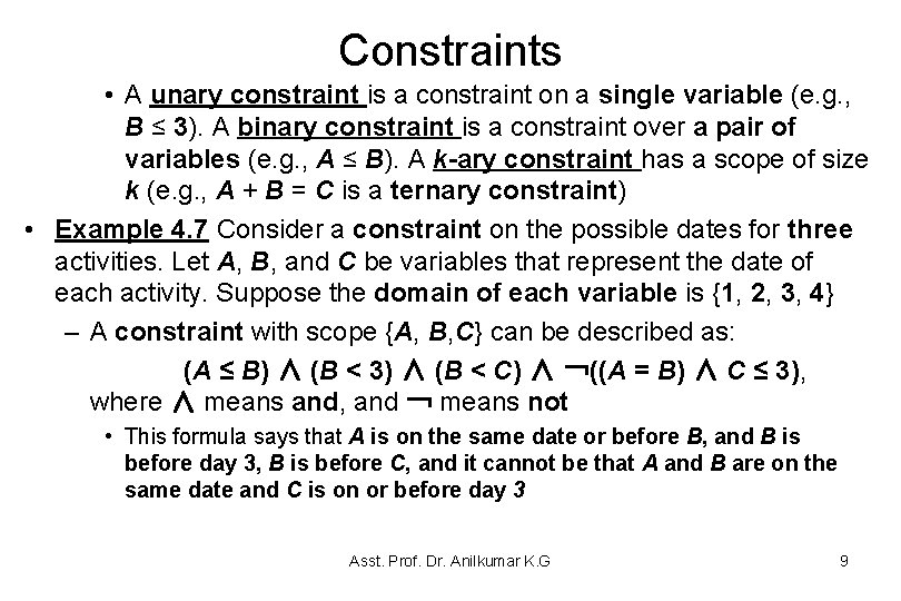
Constraints • A unary constraint is a constraint on a single variable (e. g. , B ≤ 3). A binary constraint is a constraint over a pair of variables (e. g. , A ≤ B). A k-ary constraint has a scope of size k (e. g. , A + B = C is a ternary constraint) • Example 4. 7 Consider a constraint on the possible dates for three activities. Let A, B, and C be variables that represent the date of each activity. Suppose the domain of each variable is {1, 2, 3, 4} – A constraint with scope {A, B, C} can be described as: (A ≤ B) ∧ (B < 3) ∧ (B < C) ∧ ￢((A = B) ∧ C ≤ 3), where ∧ means and, and ￢ means not • This formula says that A is on the same date or before B, and B is before day 3, B is before C, and it cannot be that A and B are on the same date and C is on or before day 3 Asst. Prof. Dr. Anilkumar K. G 9

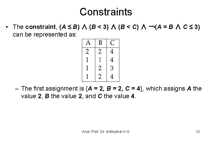
Constraints • The constraint, (A ≤ B) ∧ (B < 3) ∧ (B < C) ∧ ￢(A = B ∧ C ≤ 3) can be represented as: – The first assignment is {A = 2, B = 2, C = 4}, which assigns A the value 2, B the value 2, and C the value 4. Asst. Prof. Dr. Anilkumar K. G 10

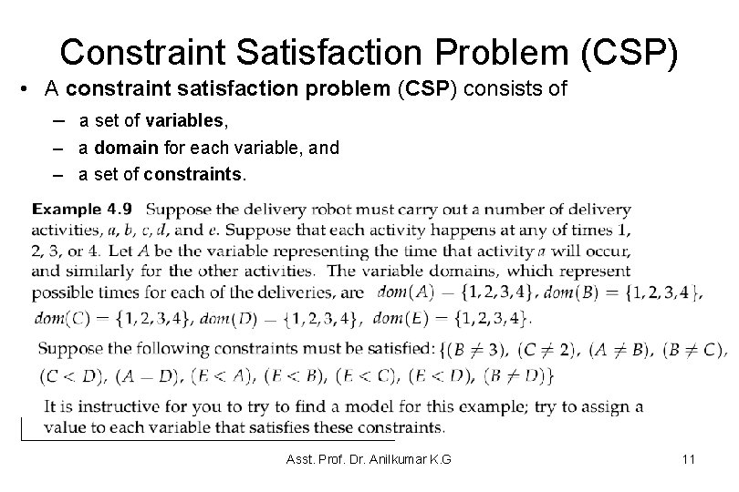
Constraint Satisfaction Problem (CSP) • A constraint satisfaction problem (CSP) consists of – a set of variables, – a domain for each variable, and – a set of constraints. Asst. Prof. Dr. Anilkumar K. G 11

Constraint Satisfaction Problem (CSP) • Given a CSP, a number of tasks are useful: – – Determine whether or not there is a model Find a model Enumerate all of the models Find a best model, based on a given measure • CSPs are very common, so it is worth trying to find efficient ways to solve them – Determining whethere is a model for a CSP with finite domains is NP-complete • a problem is NP-complete does not mean that all instances are difficult to solve Asst. Prof. Dr. Anilkumar K. G 12

Generate-and-Test Algorithm • A finite CSP could be solved by a generate-and-test algorithm • The generate-and-test algorithm used to find (best) models of the CSP problem as: – check each total assignment in turn; – if an assignment is found that satisfies all of the constraints, return that assignment. – A generate-and-test algorithm finds all the models except, • instead of returning the first model found, it saves all of the models found. • Generate-and-test algorithms assign values to all variables before checking the constraints Asst. Prof. Dr. Anilkumar K. G 13

Generate-and-Test Algorithm • Example 4. 10: In Example 4. 9, suppose the assignment space D, D = {{A = 1, B = 1, C = 1, D =1, E = 1}, {A = 1, B = 1, C = 1, D = 1, E = 2}, . . . , {A = 4, B = 4, C = 4, D = 4, E = 4}}. – In this case there are |D| = 45 (5 variables and 4 domain values) = 1, 024 different assignments to be tested. – If there were 15 variables, then there would be 415 ( = 230 = a billion) assignments to test. • This method could not work for 30 variables. • In Example 4. 9, the assignments A = 1 and B = 1 are inconsistent with the constraint A B regardless of the values of the other variables. • If each of the n variable domains has size d, then D has dn elements. • If there are e constraints, the total number of constraints tested is O(edn). As n becomes large, this very quickly becomes intractable Asst. Prof. Dr. Anilkumar K. G 14

Solving CSPs Using Search • An alternative to generate-and-test algorithms is to construct a search space as a graph search: – The nodes are assignments of values to some subset of the variables. – The neighbors of a node n are obtained by selecting a variable Y that is not assigned in node n and by having a neighbor for each assignment of a value to Y that does not violate any constraint. – The start node is the empty assignment that does not assign a value to any variables. – A goal node is a node that assigns a value to every variable. • Note that this only exists if the assignment is consistent with all of the constraints. – In this case, it is not the path from the start node that is of interest, but the goal nodes. Asst. Prof. Dr. Anilkumar K. G 15

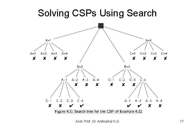
Solving CSPs Using Search • Example 4. 12: Suppose you have a very simple CSP with the variables A, B, and C, each with domain {1, 2, 3, 4}. Suppose the constraints are (A < B) (B < C). A possible search tree of the problem is shown in Figure 4. 1. In this tree, a node corresponds to all of the assignments from the root to that node. The potential nodes that are pruned because they violate constraints and are labeled with✘. – The leftmost ✘ corresponds to the assignment A =1, B = 1 (this violates the (A < B) constraint, and so it is pruned). – This CSP has four solutions (see the Figure). – The size of the search tree, and thus the efficiency of the algorithm, depends on which variable is selected at each time. – A static ordering, such as always splitting on A then B then C, is usually less efficient than the dynamic ordering. Asst. Prof. Dr. Anilkumar K. G 16

Solving CSPs Using Search Asst. Prof. Dr. Anilkumar K. G 17

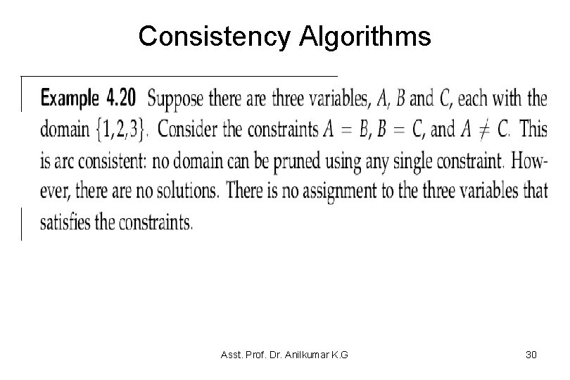
Consistency Algorithms • Example 4. 13: In Example 4. 12, the variables A and B are related by the constraint A < B. The assignment A = 4 is inconsistent with each of the possible assignments to B because dom(B) = {1, 2, 3, 4}. – In the course of the backtrack search (see Figure 4. 1), this fact is rediscovered for different assignments to B and C. – This inefficiency can be avoided by the simple expedient of deleting 4 from dom(A), once and for all. – This idea is the basis for the consistency algorithms. Asst. Prof. Dr. Anilkumar K. G 18

Consistency Algorithms • The consistency algorithms are best thought of as operating over the network of constraints formed by the CSP: – There is a node for each variable (these nodes are drawn as circles or ovals). – There is a node for each constraint (these nodes are drawn as rectangles). – Associated with each variable, X, is a set DX of possible values. • This set of values is initially the domain of the variable. – For every constraint c, and for every variable X in the scope of c, there is an arc (X, c). ´ – Such a network is called a constraint network. Asst. Prof. Dr. Anilkumar K. G 19

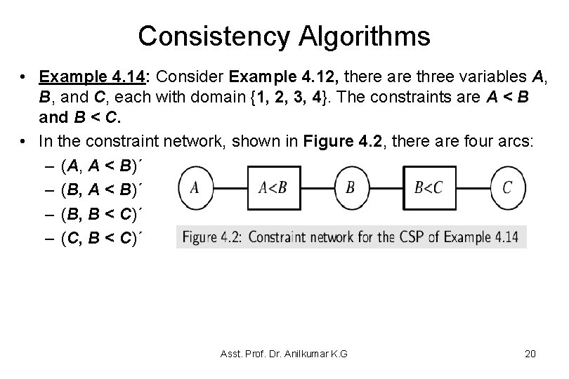
Consistency Algorithms • Example 4. 14: Consider Example 4. 12, there are three variables A, B, and C, each with domain {1, 2, 3, 4}. The constraints are A < B and B < C. • In the constraint network, shown in Figure 4. 2, there are four arcs: – (A, A < B)´ – (B, B < C)´ – (C, B < C)´ Asst. Prof. Dr. Anilkumar K. G 20

Consistency Algorithms • The generalized arc consistency (GAC) algorithm is given in Figure 4. 3. • It makes the entire network arc consistent by considering a set of potentially inconsistent arcs, the to_do arcs. • The set to_do initially consists of all the arcs in the graph. • While the set is not empty, an arc(X, c)´ is removed from the set and considered. • If the arc is not arc consistent, it is made arc consistent by pruning the domain of variable X. • All of the previously consistent arcs that could, as a result of pruning X, have become inconsistent are placed back into the set to_do. • These are the arcs(Z, c’)´, where c’ is a constraint different from c that involves X, and Z is a variable involved in c’ other than X. Asst. Prof. Dr. Anilkumar K. G 21

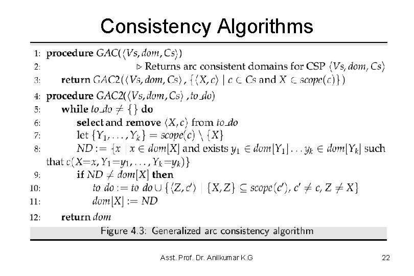
Consistency Algorithms Asst. Prof. Dr. Anilkumar K. G 22

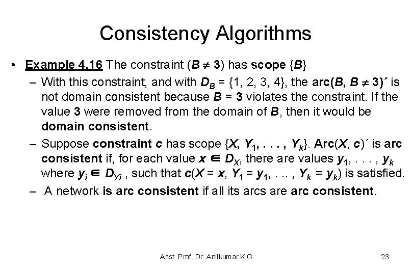
Consistency Algorithms • Example 4. 16 The constraint (B 3) has scope {B} – With this constraint, and with DB = {1, 2, 3, 4}, the arc(B, B 3)´ is not domain consistent because B = 3 violates the constraint. If the value 3 were removed from the domain of B, then it would be domain consistent. – Suppose constraint c has scope {X, Y 1, . . . , Yk}. Arc(X, c)´ is arc consistent if, for each value x ∈ DX, there are values y 1, . . . , yk where yi ∈ DYi , such that c(X = x, Y 1 = y 1, . . . , Yk = yk) is satisfied. – A network is arc consistent if all its arcs are arc consistent. Asst. Prof. Dr. Anilkumar K. G 23

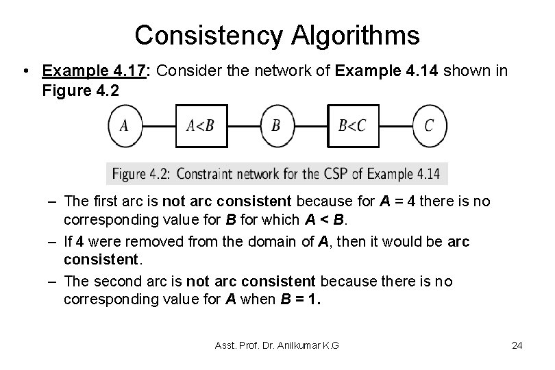
Consistency Algorithms • Example 4. 17: Consider the network of Example 4. 14 shown in Figure 4. 2 – The first arc is not arc consistent because for A = 4 there is no corresponding value for B for which A < B. – If 4 were removed from the domain of A, then it would be arc consistent. – The second arc is not arc consistent because there is no corresponding value for A when B = 1. Asst. Prof. Dr. Anilkumar K. G 24

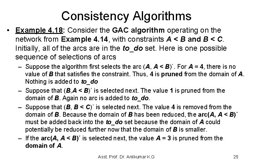
Consistency Algorithms • Example 4. 18: Consider the GAC algorithm operating on the network from Example 4. 14, with constraints A < B and B < C. Initially, all of the arcs are in the to_do set. Here is one possible sequence of selections of arcs – Suppose the algorithm first selects the arc (A, A < B)´. For A = 4, there is no value of B that satisfies the constraint. Thus, 4 is pruned from the domain of A. Nothing is added to to_do – Suppose that (B, A < B)´ is selected next. The value 1 is pruned from the domain of B. Again no arc is added to to_do. – Suppose that (B, B < C)´ is selected next. The value 4 is removed from the domain of B. Because the domain of B has been reduced, the arc(A, A < B)´ must be added back into the to_do set because the domain of A could potentially be reduced further now that the domain of B is smaller. – If the arc(A, A < B)´ is selected next, the value A = 3 is pruned from the domain of A. Asst. Prof. Dr. Anilkumar K. G 25

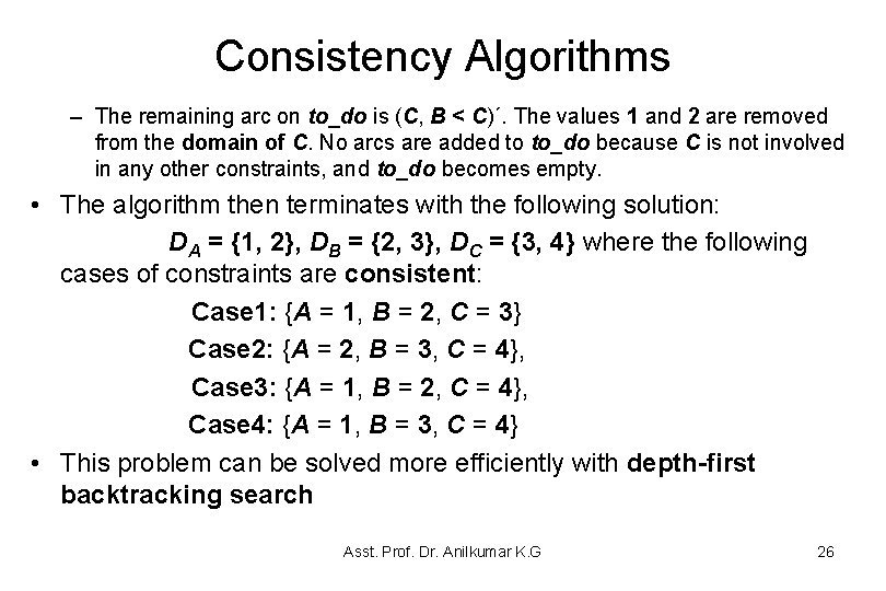
Consistency Algorithms – The remaining arc on to_do is (C, B < C)´. The values 1 and 2 are removed from the domain of C. No arcs are added to to_do because C is not involved in any other constraints, and to_do becomes empty. • The algorithm then terminates with the following solution: DA = {1, 2}, DB = {2, 3}, DC = {3, 4} where the following cases of constraints are consistent: Case 1: {A = 1, B = 2, C = 3} Case 2: {A = 2, B = 3, C = 4}, Case 3: {A = 1, B = 2, C = 4}, Case 4: {A = 1, B = 3, C = 4} • This problem can be solved more efficiently with depth-first backtracking search Asst. Prof. Dr. Anilkumar K. G 26

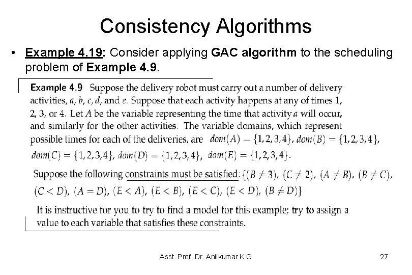
Consistency Algorithms • Example 4. 19: Consider applying GAC algorithm to the scheduling problem of Example 4. 9. Asst. Prof. Dr. Anilkumar K. G 27

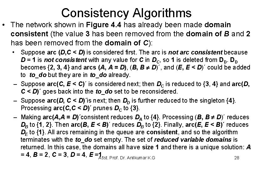
Consistency Algorithms • The network shown in Figure 4. 4 has already been made domain consistent (the value 3 has been removed from the domain of B and 2 has been removed from the domain of C): • Suppose arc (D, C < D) is considered first. The arc is not arc consistent because D = 1 is not consistent with any value for C in DC, so 1 is deleted from DD. DD becomes {2, 3, 4} and arcs (A, A = D), (B, B D)´, and (E, E < D)´ could be added to to_do but they are in to_do already. – Suppose arc(C, E < C)´ is considered next; then DC is reduced to {3, 4} and arc(D, C < D)´ goes back into the to_do set to be reconsidered. – Suppose arc(D, C < D)´is next; then DD is further reduced to the singleton {4}. Processing arc(C, C < D)´ prunes DC to {3}. – Making arc(A, A = D)´consistent reduces DA to {4}. Processing (B, B D)´ reduces DB to {1, 2}. Then arc(B, E < B)´ reduces DB to {2}. Finally, arc(E, E < B)´ reduces DE to {1}. All arcs remaining in the queue are consistent, and so the algorithm terminates with the to_do set empty. The set of reduced variable domains is returned. In this case, the domains all have size 1 and there is a unique solution: A = 4, B = 2, C = 3, D = 4, E =1. Asst. Prof. Dr. Anilkumar K. G 28

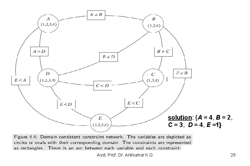
solution: {A = 4, B = 2, C = 3, D = 4, E =1} Asst. Prof. Dr. Anilkumar K. G 29

Consistency Algorithms Asst. Prof. Dr. Anilkumar K. G 30

Domain Splitting • Another method for simplifying the CSP network is domain splitting – The idea is to split a problem into a number of disjoint cases and solve each case separately. – The set of all solutions to the initial problem is the union of the solutions to each case. • In the simplest case, assume there is a binary variable X with domain {t, f }. – All of the solutions either have X = t or X = f. – One way to find all of the solutions is to set X = t, find all of the solutions with this assignment, and then assign X = f if not. – Assigning a value to a variable gives a smaller reduced problem to solve. – If we only want to find one solution, we can look for the solutions with X = t, and if we do not find any, we can look for the solutions with X = f. Asst. Prof. Dr. Anilkumar K. G 31

Domain Splitting • For example if the domain of A is {1, 2, 3, 4}, there a number of ways to split it: – Split the domain into a case for each value. Such as, split A into the four cases A = 1, A = 2, A = 3, and A = 4. – Always split the domain into two disjoint non-empty subsets. • For example, split A into the two cases: A ∈ {1, 2} and A ∈ {3, 4}. • The first approach makes more progress with one split, but the second may allow for more pruning with fewer steps • For example, if the same values for B can be pruned whether A is 1 or 2, the second case allows this fact to be discovered once and not have to be rediscovered for each element of A. • One effective way to solve a CSP is to use arc consistency to simplify the network before each step of domain splitting. Asst. Prof. Dr. Anilkumar K. G 32

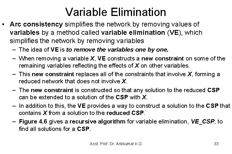
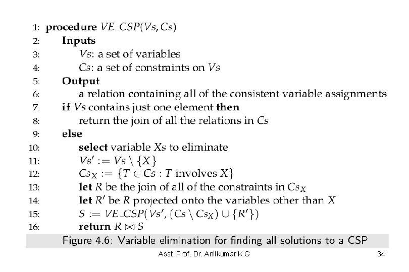
Variable Elimination • Arc consistency simplifies the network by removing values of variables by a method called variable elimination (VE), which simplifies the network by removing variables – The idea of VE is to remove the variables one by one. – When removing a variable X, VE constructs a new constraint on some of the remaining variables reflecting the effects of X on other variables. – This new constraint replaces all of the constraints that involve X, forming a reduced network that does not involve X. – The new constraint is constructed so that any solution to the reduced CSP can be extended to a solution of the CSP with X. – In addition to this, the VE provides a way to construct a solution to the CSP that contains X from a solution to the reduced CSP. – Figure 4. 6 gives a recursive algorithm for variable elimination, VE_CSP, to find all solutions for a CSP. Asst. Prof. Dr. Anilkumar K. G 33

Asst. Prof. Dr. Anilkumar K. G 34

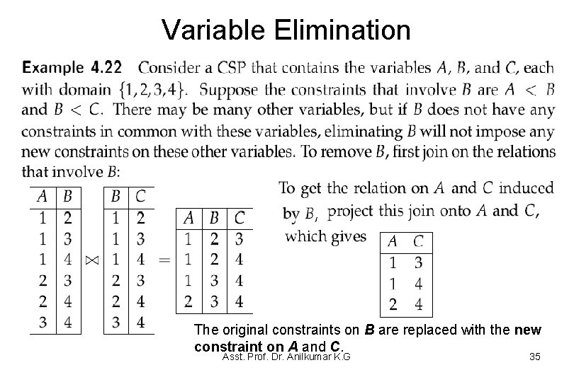
Variable Elimination The original constraints on B are replaced with the new constraint on A and C. Asst. Prof. Dr. Anilkumar K. G 35

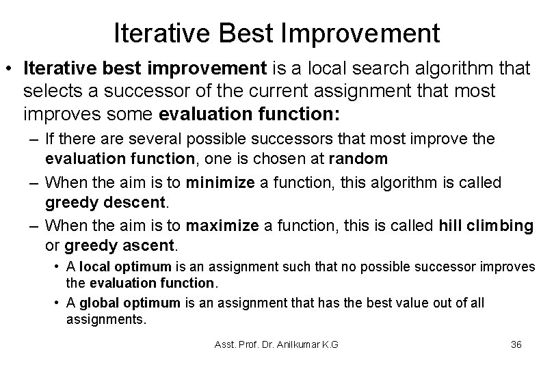
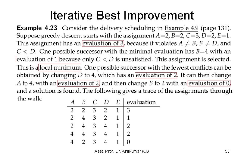
Iterative Best Improvement • Iterative best improvement is a local search algorithm that selects a successor of the current assignment that most improves some evaluation function: – If there are several possible successors that most improve the evaluation function, one is chosen at random – When the aim is to minimize a function, this algorithm is called greedy descent. – When the aim is to maximize a function, this is called hill climbing or greedy ascent. • A local optimum is an assignment such that no possible successor improves the evaluation function. • A global optimum is an assignment that has the best value out of all assignments. Asst. Prof. Dr. Anilkumar K. G 36

Iterative Best Improvement Asst. Prof. Dr. Anilkumar K. G 37

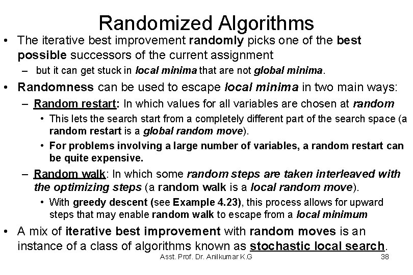
Randomized Algorithms • The iterative best improvement randomly picks one of the best possible successors of the current assignment – but it can get stuck in local minima that are not global minima. • Randomness can be used to escape local minima in two main ways: – Random restart: In which values for all variables are chosen at random • This lets the search start from a completely different part of the search space (a random restart is a global random move). • For problems involving a large number of variables, a random restart can be quite expensive. – Random walk: In which some random steps are taken interleaved with the optimizing steps (a random walk is a local random move). • With greedy descent (see Example 4. 23), this process allows for upward steps that may enable random walk to escape from a local minimum • A mix of iterative best improvement with random moves is an instance of a class of algorithms known as stochastic local search. Asst. Prof. Dr. Anilkumar K. G 38

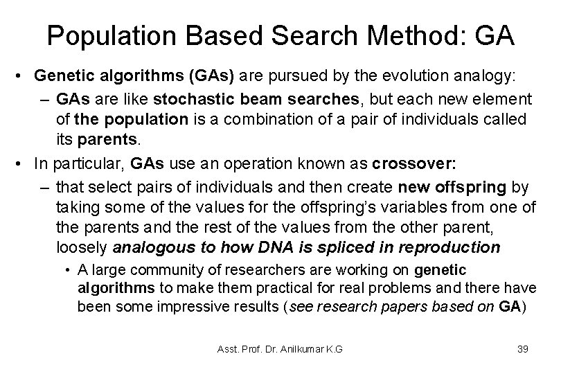
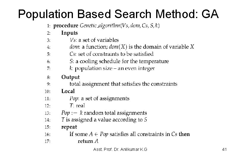
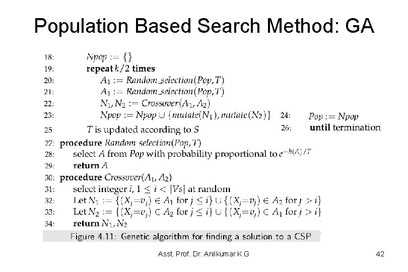
Population Based Search Method: GA • Genetic algorithms (GAs) are pursued by the evolution analogy: – GAs are like stochastic beam searches, but each new element of the population is a combination of a pair of individuals called its parents. • In particular, GAs use an operation known as crossover: – that select pairs of individuals and then create new offspring by taking some of the values for the offspring’s variables from one of the parents and the rest of the values from the other parent, loosely analogous to how DNA is spliced in reproduction • A large community of researchers are working on genetic algorithms to make them practical for real problems and there have been some impressive results (see research papers based on GA) Asst. Prof. Dr. Anilkumar K. G 39

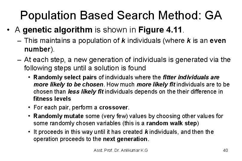
Population Based Search Method: GA • A genetic algorithm is shown in Figure 4. 11. – This maintains a population of k individuals (where k is an even number). – At each step, a new generation of individuals is generated via the following steps until a solution is found • Randomly select pairs of individuals where the fitter individuals are more likely to be chosen. How much more likely fit individuals are to be chosen than less likely fit individuals depends on their difference in fitness levels • For each pair, perform a crossover. • Randomly mutate some (very few) values by choosing other values for some randomly chosen variables (this is a random walk step) • It proceeds in this way until it has created k individuals, and then the operation proceeds to the next generation. Asst. Prof. Dr. Anilkumar K. G 40

Population Based Search Method: GA Asst. Prof. Dr. Anilkumar K. G 41

Population Based Search Method: GA Asst. Prof. Dr. Anilkumar K. G 42

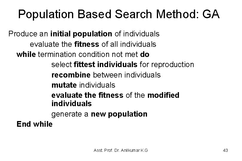
Population Based Search Method: GA Produce an initial population of individuals evaluate the fitness of all individuals while termination condition not met do select fittest individuals for reproduction recombine between individuals mutate individuals evaluate the fitness of the modified individuals generate a new population End while Asst. Prof. Dr. Anilkumar K. G 43

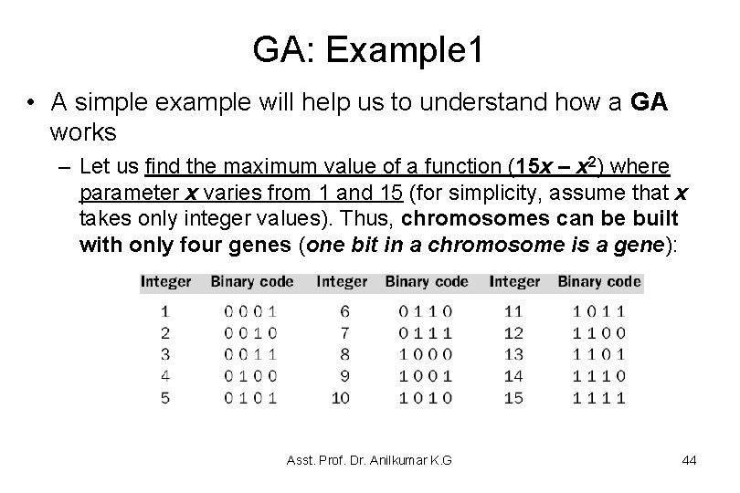
GA: Example 1 • A simple example will help us to understand how a GA works – Let us find the maximum value of a function (15 x – x 2) where parameter x varies from 1 and 15 (for simplicity, assume that x takes only integer values). Thus, chromosomes can be built with only four genes (one bit in a chromosome is a gene): Asst. Prof. Dr. Anilkumar K. G 44

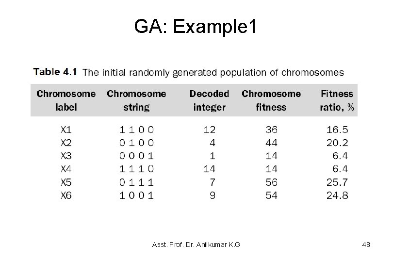
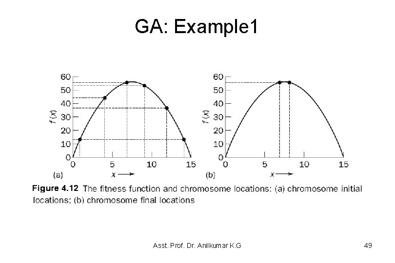
GA: Example 1 – Suppose that the size of the chromosome population N is 6 (randomly generate six, 4 -bit values), the crossover probability pc equals 0. 7 (4/6 0. 7) and the mutation probability pm equals 0. 001 (1 in 1000 generations). The fitness function of the problem is defined by: f(x) = 15 x – x 2 – The GA creates an initial population of chromosomes by filling six 4 -bit strings with randomly generated 1 s and 0 s – The initial population might look like that shown in Table 4. 1 – The chromosomes initial locations on the fitness function are illustrated in Figure 4. 12 – A real practical problem would typically have a population of thousands of chromosomes Asst. Prof. Dr. Anilkumar K. G 45

GA: Example 1 – The next step is to calculate the fitness of each individual chromosome. The results are shown in Table 4. 1 – The average fitness of the initial population is 36 – The fitness ratio = (fitness/total fitness) x 100 for e. g. . , (36/218)*100 = 16. 5% • In order to improve it, the initial population is modified by using the genetic operators such as selection, cross over and mutation • In natural selection, only the fittest species can survive, breed and thereby pass their genes on to the next generation • GA uses the similar natural selection style approach, but unlike nature, the size of the chromosome population remains unchanged from one generation to the next Asst. Prof. Dr. Anilkumar K. G 46

GA: Example 2 • The GA cycle is illustrated in this example for maximizing a function f(x) = x 2 in the interval 0 x 31 • In this example the fitness function is f(x) itself – The larger is the functional value, the better is the fitness of the string • In this example, we start with 4 initial chromosomes • The fitness value of the strings and the percentage fitness of the total are estimated in Table 4. 2 – Since fitness of the second string is large, select 2 copies of the second string and one each for the first and fourth string in the crossover pool Asst. Prof. Dr. Anilkumar K. G 47

GA: Example 1 Asst. Prof. Dr. Anilkumar K. G 48

GA: Example 1 Asst. Prof. Dr. Anilkumar K. G 49

GA: Example 1 • The last column in Table 4. 1 shows the ratio of the individual chromosome’s fitness to the population’s total fitness – This ratio determines the chromosome’s chance of being selected for mating • Thus the chromosome X 5 and X 6 stand a fair chance, while the chromosomes X 3 and X 4 have a very low probability of being selected for crossover • As a result, the chromosome’s average fitness improves from one generation to the next Asst. Prof. Dr. Anilkumar K. G 50

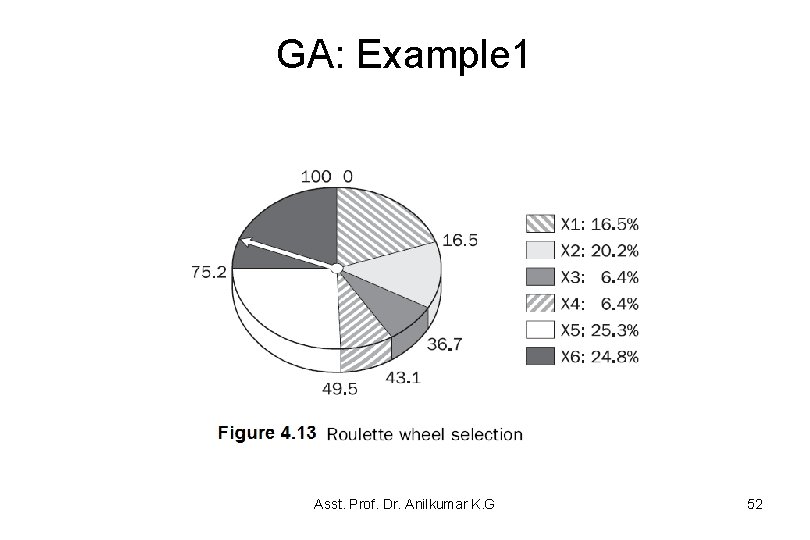
GA: Example 1 • One of the most commonly used chromosome selection techniques is the roulette wheel selection • Figure 4. 13 illustrates the roulette wheel for the previous problem example – See each chromosome is given a slice of a circular roulette wheel – The area of the slice within the wheel is equal to the chromosome fitness ratio (see Table 4. 1). For instance, the chromosomes X 5 and X 6 (the most fit chromosomes) occupy the largest areas, whereas the chromosomes X 3 and X 4 (least fit) have much smaller segments in the roulette wheel Asst. Prof. Dr. Anilkumar K. G 51

GA: Example 1 Asst. Prof. Dr. Anilkumar K. G 52

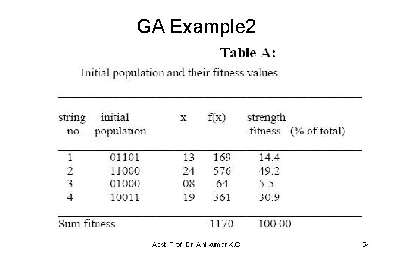
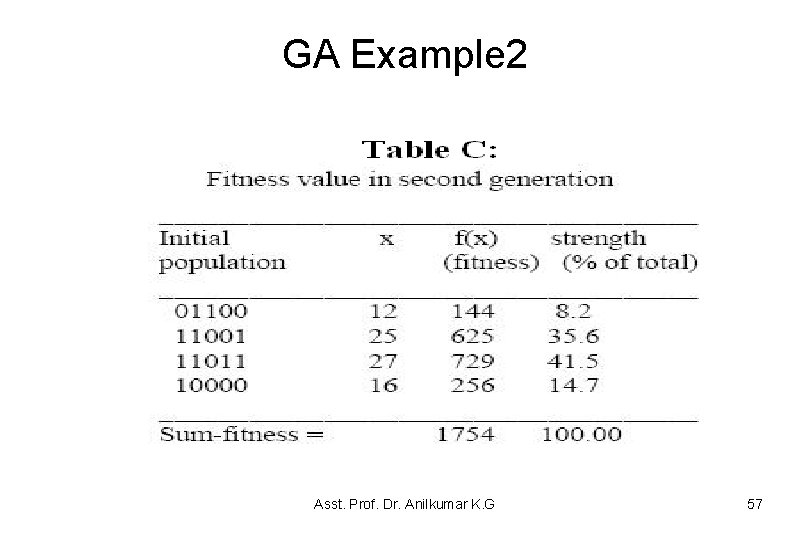
GA Example 2 • The GA cycle is illustrated in this example for maximizing a function f(x) = x 2 in the interval 0 x 31 • In this example the fitness function is f(x) itself – The larger is the functional value, the better is the fitness of the string • In this example, we start with 4 initial chromosomes • The fitness value of the strings and the percentage fitness of the total are estimated in Table A – Since fitness of the second string is large, select 2 copies of the second string and one each for the first and fourth string in the crossover pool Asst. Prof. Dr. Anilkumar K. G 53

GA Example 2 Asst. Prof. Dr. Anilkumar K. G 54

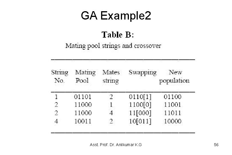
GA Example 2 • The selection of the partners in the crossover pool is also done randomly – Here in table B, we selected partner of string 1 to be the 2 nd string and partner of 4 th string to be the 2 nd string • The crossover points for the first-second and secondfourth strings have been selected and are shown in table B • The second generation of the population without mutation in the first generation is presented in table C Asst. Prof. Dr. Anilkumar K. G 55

GA Example 2 Asst. Prof. Dr. Anilkumar K. G 56

GA Example 2 Asst. Prof. Dr. Anilkumar K. G 57

GA Example 3 • Let us consider a diophantine equation (the diophantine equation is an indeterminate polynomial equation that allows the variables to be integers only ) : a + 2 b + 3 c + 4 d = 30, where a, b, c and d are three positive integer variables • Using the GA, all that is needed is a solution: (a? , b ? , c? , d? ) – Why not just use a brute force method to find its solution? (plug in every possible value for (a, b, c, d) given the constraints 1 (a, b, c, d) 30)? • For the given problem, the architecture of GA allows for a solution to be reached quicker since “better” solutions have a better chance of surviving and procreating as opposed to randomly throwing out solutions and seeing which ones work Asst. Prof. Dr. Anilkumar K. G 58

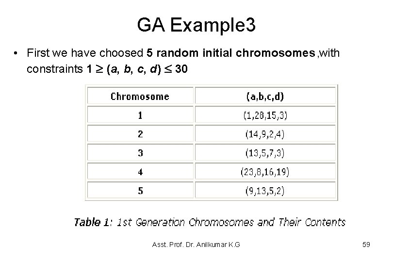
GA Example 3 • First we have choosed 5 random initial chromosomes , with constraints 1 (a, b, c, d) 30 Asst. Prof. Dr. Anilkumar K. G 59

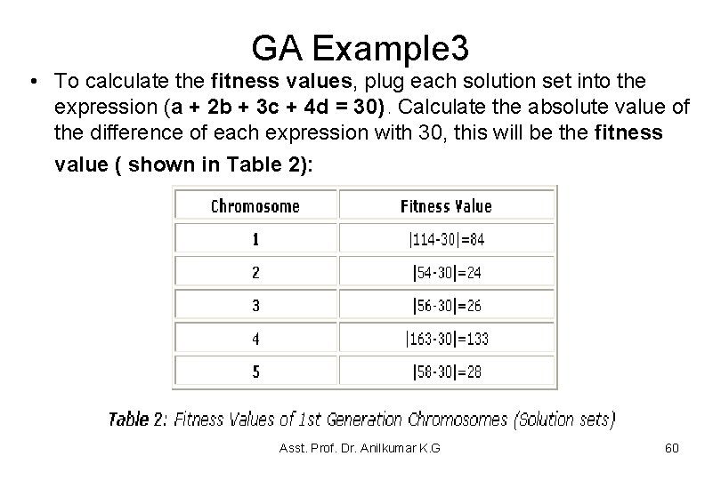
GA Example 3 • To calculate the fitness values, plug each solution set into the expression (a + 2 b + 3 c + 4 d = 30). Calculate the absolute value of the difference of each expression with 30, this will be the fitness value ( shown in Table 2): Asst. Prof. Dr. Anilkumar K. G 60

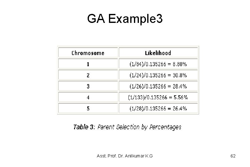
GA Example 3 • Since values that are lower are closer to the desired answer (30), these values are more desirable – In this case, higher fitness values are not desirable • In order to create a system where chromosomes with more desirable fitness values are more likely to be chosen as parents. • Table 3 shows the percentages that each chromosome has of being picked – One solution is to take the sum of the multiplicative inverses of the fitness values (1/84 + 1/26 + 1/133 + 1/28 = 0. 135266), and calculate the percentages from there (see Table 3) Asst. Prof. Dr. Anilkumar K. G 61

GA Example 3 Asst. Prof. Dr. Anilkumar K. G 62

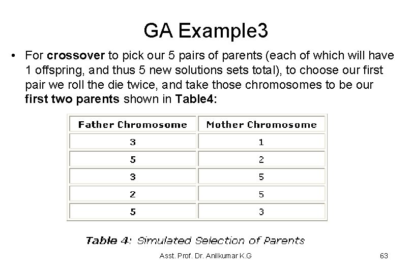
GA Example 3 • For crossover to pick our 5 pairs of parents (each of which will have 1 offspring, and thus 5 new solutions sets total), to choose our first pair we roll the die twice, and take those chromosomes to be our first two parents shown in Table 4: Asst. Prof. Dr. Anilkumar K. G 63

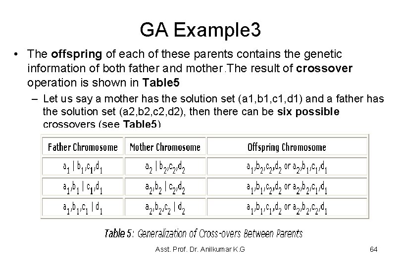
GA Example 3 • The offspring of each of these parents contains the genetic information of both father and mother. The result of crossover operation is shown in Table 5 – Let us say a mother has the solution set (a 1, b 1, c 1, d 1) and a father has the solution set (a 2, b 2, c 2, d 2), then there can be six possible crossovers (see Table 5) Asst. Prof. Dr. Anilkumar K. G 64

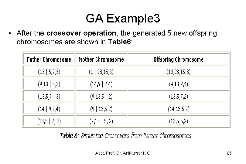
GA Example 3 • After the crossover operation, the generated 5 new offspring chromosomes are shown in Table 6: Asst. Prof. Dr. Anilkumar K. G 65

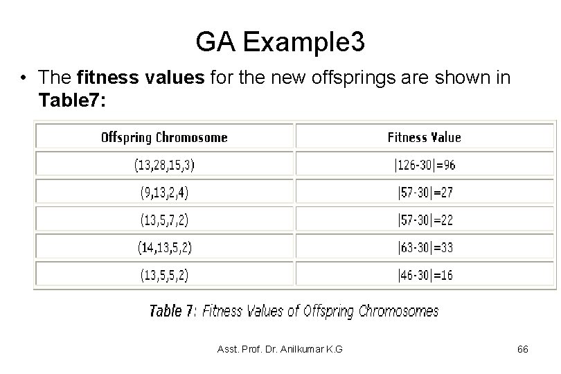
GA Example 3 • The fitness values for the new offsprings are shown in Table 7: Asst. Prof. Dr. Anilkumar K. G 66

GA Example 3 • The average fitness value for the offspring chromosomes were 38. 8, while the average fitness value for the parent chromosomes were 59. 4 – Of course, the next generation (the offspring)are supposed to mutate, that is, for example we can change one of the values in the ordered quadruple of each chromosome to some random integer between 1 and 30 • Progressing at this rate, one chromosome should eventually reach a fitness level of 0 eventually, that is when a solution is found. – For systems where the population is larger (say 50, instead of 5), the fitness levels should more steadily and stable approach the desired level. Asst. Prof. Dr. Anilkumar K. G 67

Optimization • From a preference relation over possible worlds to find a best possible world according to the preference is called optimization • An optimization problem is given – set of variables, each with an associated domain – an objective function that maps total assignments to real numbers, and – an optimality criterion, which is typically to find a total assignment that minimizes or maximizes the objective function • The aim is to find a total assignment that is optimal according to the optimality criterion. • For concreteness, we assume that the optimality criterion is to minimize the objective function. Asst. Prof. Dr. Anilkumar K. G 68

Optimization • In a constraint optimization problem, the objective function is factored into a set of soft constraints • A soft constraint has a scope that is a set of variables. • The soft constraint is a function from the domains of the variables in its scope into a real number, a cost. • A typical optimality criterion is to choose a total assignment that minimizes the sum of the costs of the soft constraints. Asst. Prof. Dr. Anilkumar K. G 69

Gradient Descent • For optimization, the evaluation function is continuous and differentiable, – gradient descent can be used to find a minimum value, and – gradient ascent can be used to find a maximum value. • Gradient descent is like walking downhill and always taking a step in the direction that goes down the most: – The general idea is that the successor of a total assignment is a step downhill in proportion to the slope of the evaluation function h. – Thus, gradient descent takes steps in each direction proportional to the negative of the partial derivative in that direction. Asst. Prof. Dr. Anilkumar K. G 70

Gradient Descent • Gradient descent is commonly used as an optimization algorithm that iteratively updates the learnable parameters, – i. e. , kernels, weights, and biases, of a neural network so as to minimize the loss • The gradient of the loss function provides us the direction in which the function has the steepest rate of increase, and each learnable parameter is updated in the negative direction of the gradient with an arbitrary step size determined based on a hyperparameter called learning rate (see Figure 8. 2). • Gradient is basically defined as the slope of the curve and is the derivative of the activation function. Asst. Prof. Dr. Anilkumar K. G 71

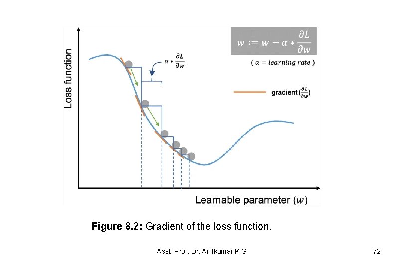
Figure 8. 2: Gradient of the loss function. Asst. Prof. Dr. Anilkumar K. G 72

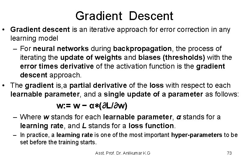
Gradient Descent • Gradient descent is an iterative approach for error correction in any learning model – For neural networks during backpropagation, the process of iterating the update of weights and biases (thresholds) with the error times derivative of the activation function is the gradient descent approach. • The gradient is, a partial derivative of the loss with respect to each learnable parameter, and a single update of a parameter as follows: w: = w − α∗(∂L/∂w) – Where w stands for each learnable parameter, α stands for a learning rate, and L stands for a loss function. – In practice, a learning rate is one of the most important hyper-parameters to be set before the training starts. Asst. Prof. Dr. Anilkumar K. G 73

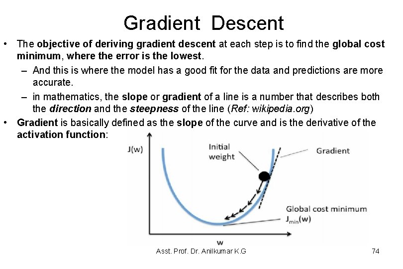
Gradient Descent • The objective of deriving gradient descent at each step is to find the global cost minimum, where the error is the lowest. – And this is where the model has a good fit for the data and predictions are more accurate. – in mathematics, the slope or gradient of a line is a number that describes both the direction and the steepness of the line (Ref: wikipedia. org) • Gradient is basically defined as the slope of the curve and is the derivative of the activation function: Asst. Prof. Dr. Anilkumar K. G 74

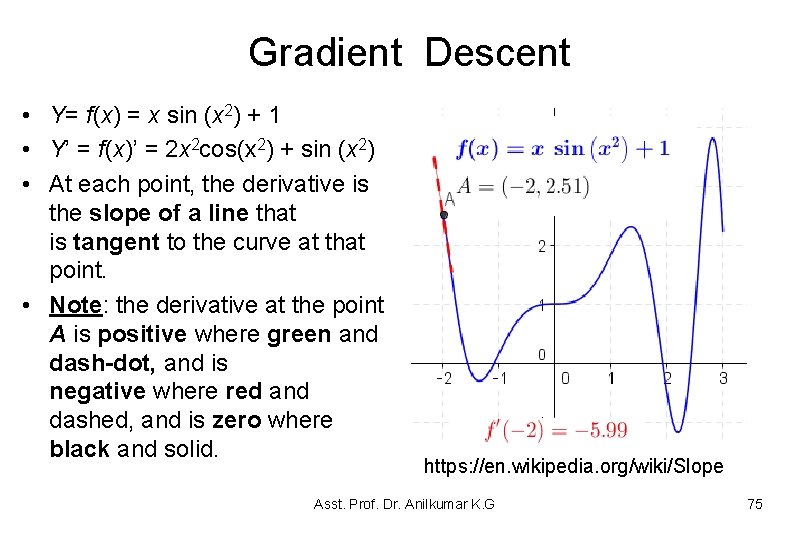
Gradient Descent • Y= f(x) = x sin (x 2) + 1 • Y’ = f(x)’ = 2 x 2 cos(x 2) + sin (x 2) • At each point, the derivative is the slope of a line that is tangent to the curve at that point. • Note: the derivative at the point A is positive where green and dash-dot, and is negative where red and dashed, and is zero where black and solid. https: //en. wikipedia. org/wiki/Slope Asst. Prof. Dr. Anilkumar K. G 75

Gradient Descent • Gradient descent can be performed either for the full batch or stochastic. – In Neural net learning, the full batch gradient descent, is the gradient is computed with the full training dataset, whereas – In Stochastic Gradient Descent (SGD) takes a single sample for gradient calculation • It can also take mini-batches and perform the calculations. • One advantage of SGD is faster computation of gradients. Asst. Prof. Dr. Anilkumar K. G 76

Gradient descent • In gradient descent optimization method, all training samples used for initial dataset training: – The advantage is that the global optimal solution is obtained when training all samples, which is easy to calculate in parallel. – The disadvantage is that when the number of training samples is large, the training process will be slow. Asst. Prof. Anilkumar K. G, Ph. D 77