Chapter 4 Probability The Study of Randomness Lecture

Chapter 4 Probability: The Study of Randomness 4. 1 Randomness 4. 2 Probability Models 4. 3 Random Variables 4. 4 Means and Variances of Random Variables 4. 5 General Probability Rules* 2

4. 1 Randomness § The language of probability § Thinking about randomness § The uses of probability 3

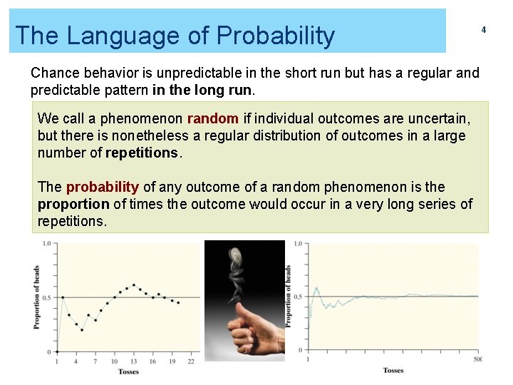
The Language of Probability 4 Chance behavior is unpredictable in the short run but has a regular and predictable pattern in the long run. We call a phenomenon random if individual outcomes are uncertain, but there is nonetheless a regular distribution of outcomes in a large number of repetitions. The probability of any outcome of a random phenomenon is the proportion of times the outcome would occur in a very long series of repetitions.

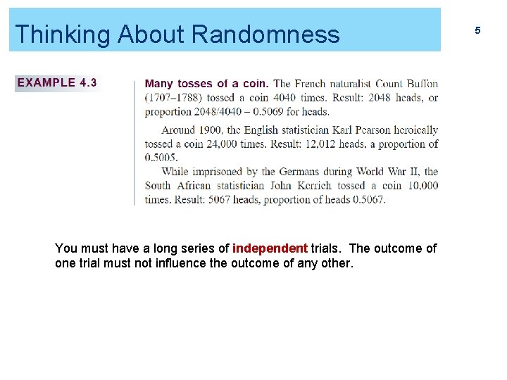
Thinking About Randomness You must have a long series of independent trials. The outcome of one trial must not influence the outcome of any other. 5

Uses of Probability q The origins of probability were seventeenth-century games of chance. q In the eighteenth and nineteenth century, careful measurements in astronomy and surveying led to further advances in probability due to distributions that arise from random sampling. q Modern applications of probability apply to such diverse fields as § § § Traffic flows Genetic makeups of a population Energy states of subatomic particles Spread of epidemics or tweets Returns on risky investments 6

4. 2 Probability Models § Sample spaces § Probability rules § Assigning probabilities: finite outcomes § Assigning probabilities: equally likely outcomes § Independence and the multiplication rule § Applying the rules 7

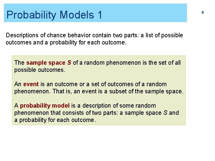
Probability Models 1 Descriptions of chance behavior contain two parts: a list of possible outcomes and a probability for each outcome. The sample space S of a random phenomenon is the set of all possible outcomes. An event is an outcome or a set of outcomes of a random phenomenon. That is, an event is a subset of the sample space. A probability model is a description of some random phenomenon that consists of two parts: a sample space S and a probability for each outcome. 8

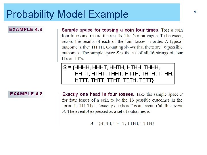
Probability Model Example S = {HHHH, HHHT, HHTH, HTHH, THHH, HHTT, HTHT, THHT, HTTH, THTH, TTHH, HTTT, THTT, TTHT, TTTH, TTTT} 9

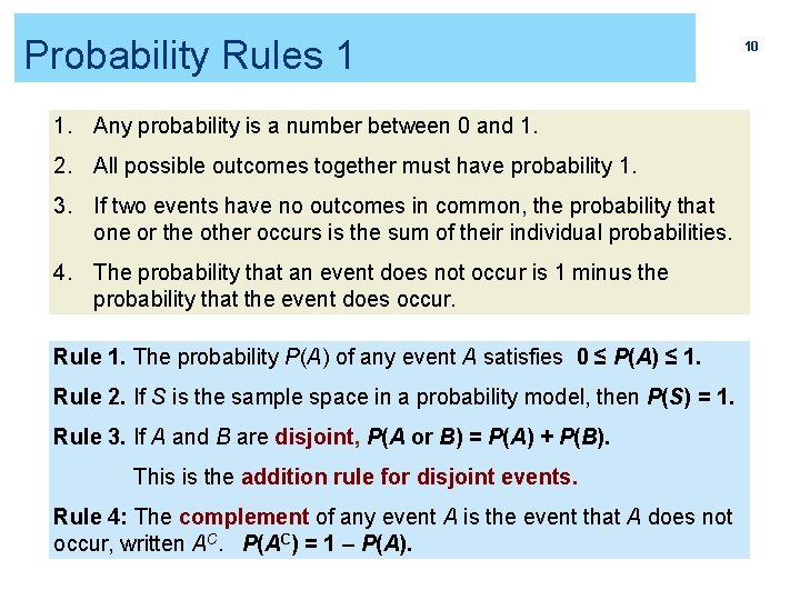
Probability Rules 1 1. Any probability is a number between 0 and 1. 2. All possible outcomes together must have probability 1. 3. If two events have no outcomes in common, the probability that one or the other occurs is the sum of their individual probabilities. 4. The probability that an event does not occur is 1 minus the probability that the event does occur. Rule 1. The probability P(A) of any event A satisfies 0 ≤ P(A) ≤ 1. Rule 2. If S is the sample space in a probability model, then P(S) = 1. Rule 3. If A and B are disjoint, P(A or B) = P(A) + P(B). This is the addition rule for disjoint events. Rule 4: The complement of any event A is the event that A does not occur, written AC. P(AC) = 1 – P(A). 10

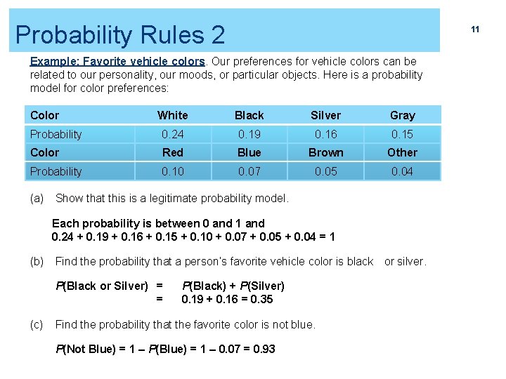
Probability Rules 2 11 Example: Favorite vehicle colors. Our preferences for vehicle colors can be related to our personality, our moods, or particular objects. Here is a probability model for color preferences: Color White Black Silver Gray Probability 0. 24 0. 19 0. 16 0. 15 Color Red Blue Brown Other Probability 0. 10 0. 07 0. 05 0. 04 (a) Show that this is a legitimate probability model. Each probability is between 0 and 1 and 0. 24 + 0. 19 + 0. 16 + 0. 15 + 0. 10 + 0. 07 + 0. 05 + 0. 04 = 1 (b) Find the probability that a person’s favorite vehicle color is black or silver. P(Black or Silver) = = (c) P(Black) + P(Silver) 0. 19 + 0. 16 = 0. 35 Find the probability that the favorite color is not blue. P(Not Blue) = 1 – P(Blue) = 1 – 0. 07 = 0. 93

Venn Diagrams 12

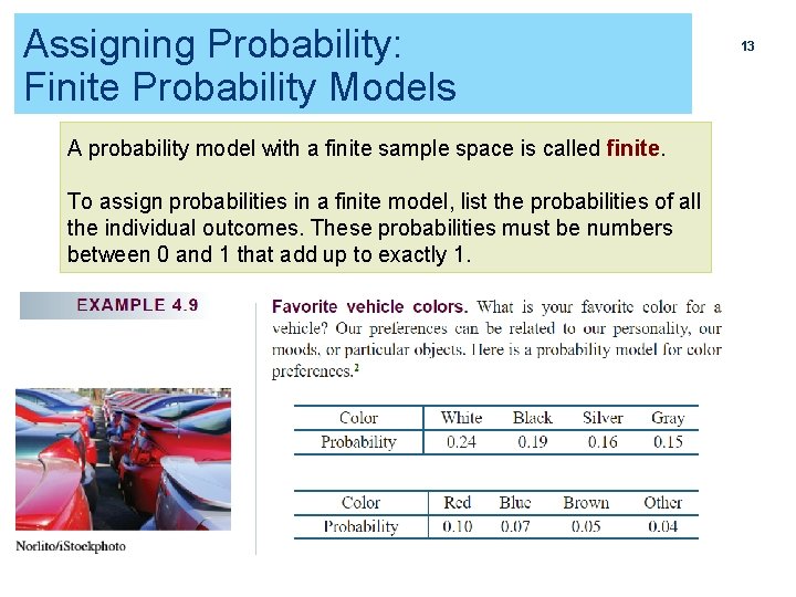
Assigning Probability: Finite Probability Models A probability model with a finite sample space is called finite. To assign probabilities in a finite model, list the probabilities of all the individual outcomes. These probabilities must be numbers between 0 and 1 that add up to exactly 1. 13

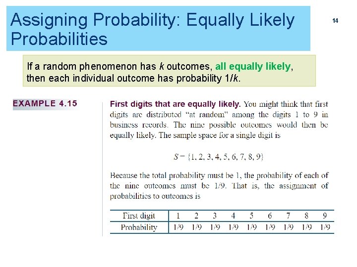
Assigning Probability: Equally Likely Probabilities If a random phenomenon has k outcomes, all equally likely, then each individual outcome has probability 1/k. 14

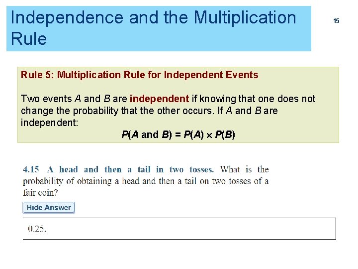
Independence and the Multiplication Rule 5: Multiplication Rule for Independent Events Two events A and B are independent if knowing that one does not change the probability that the other occurs. If A and B are independent: P(A and B) = P(A) P(B) 15

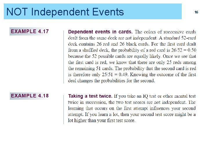
NOT Independent Events 16

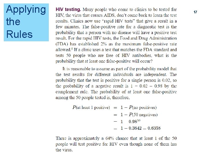
Applying the Rules 17

4. 3 Random Variables § Random variable § Discrete random variables § Continuous random variables § Normal distributions as probability distributions 18

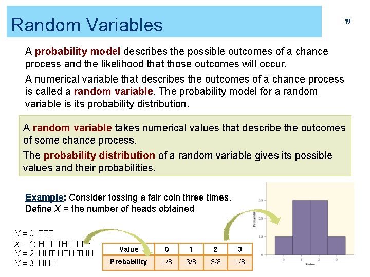
Random Variables 19 A probability model describes the possible outcomes of a chance process and the likelihood that those outcomes will occur. A numerical variable that describes the outcomes of a chance process is called a random variable. The probability model for a random variable is its probability distribution. A random variable takes numerical values that describe the outcomes of some chance process. The probability distribution of a random variable gives its possible values and their probabilities. Example: Consider tossing a fair coin three times. Define X = the number of heads obtained X = 0: TTT X = 1: HTT THT TTH X = 2: HHT HTH THH X = 3: HHH Value 0 1 2 3 Probability 1/8 3/8 1/8

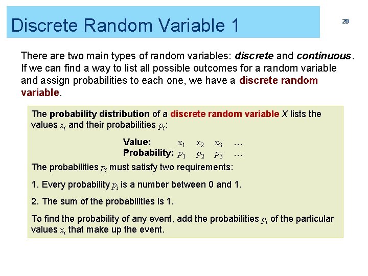
Discrete Random Variable 1 20 There are two main types of random variables: discrete and continuous. If we can find a way to list all possible outcomes for a random variable and assign probabilities to each one, we have a discrete random variable. The probability distribution of a discrete random variable X lists the values xi and their probabilities pi: Value: x 1 Probability: p 1 x 2 p 2 x 3 p 3 … … The probabilities pi must satisfy two requirements: 1. Every probability pi is a number between 0 and 1. 2. The sum of the probabilities is 1. To find the probability of any event, add the probabilities pi of the particular values xi that make up the event.

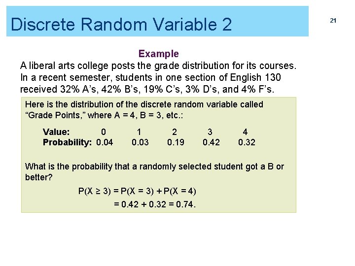
Discrete Random Variable 2 21 Example A liberal arts college posts the grade distribution for its courses. In a recent semester, students in one section of English 130 received 32% A’s, 42% B’s, 19% C’s, 3% D’s, and 4% F’s. Here is the distribution of the discrete random variable called “Grade Points, ” where A = 4, B = 3, etc. : Value: 0 Probability: 0. 04 1 0. 03 2 0. 19 3 0. 42 4 0. 32 What is the probability that a randomly selected student got a B or better? P(X ≥ 3) = P(X = 3) + P(X = 4) = 0. 42 + 0. 32 = 0. 74.

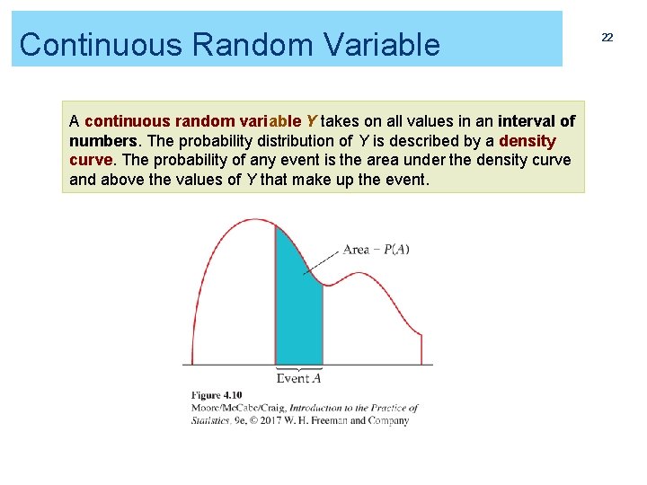
Continuous Random Variable A continuous random variable Y takes on all values in an interval of numbers. The probability distribution of Y is described by a density curve. The probability of any event is the area under the density curve and above the values of Y that make up the event. 22

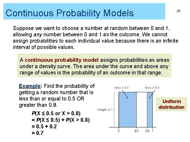
Continuous Probability Models 23 Suppose we want to choose a number at random between 0 and 1, allowing any number between 0 and 1 as the outcome. We cannot assign probabilities to each individual value because there is an infinite interval of possible values. A continuous probability model assigns probabilities as areas under a density curve. The area under the curve and above any range of values is the probability of an outcome in that range. Example: Find the probability of getting a random number that is less than or equal to 0. 5 OR greater than 0. 8. P(X ≤ 0. 5 or X > 0. 8) = P(X ≤ 0. 5) + P(X > 0. 8) = 0. 5 + 0. 2 = 0. 7 Uniform distribution

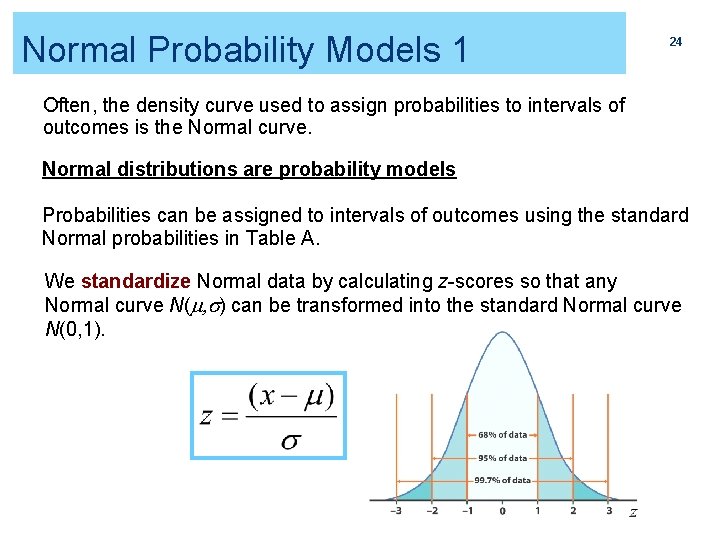
Normal Probability Models 1 24 Often, the density curve used to assign probabilities to intervals of outcomes is the Normal curve. Normal distributions are probability models Probabilities can be assigned to intervals of outcomes using the standard Normal probabilities in Table A. We standardize Normal data by calculating z-scores so that any Normal curve N(m, s) can be transformed into the standard Normal curve N(0, 1).

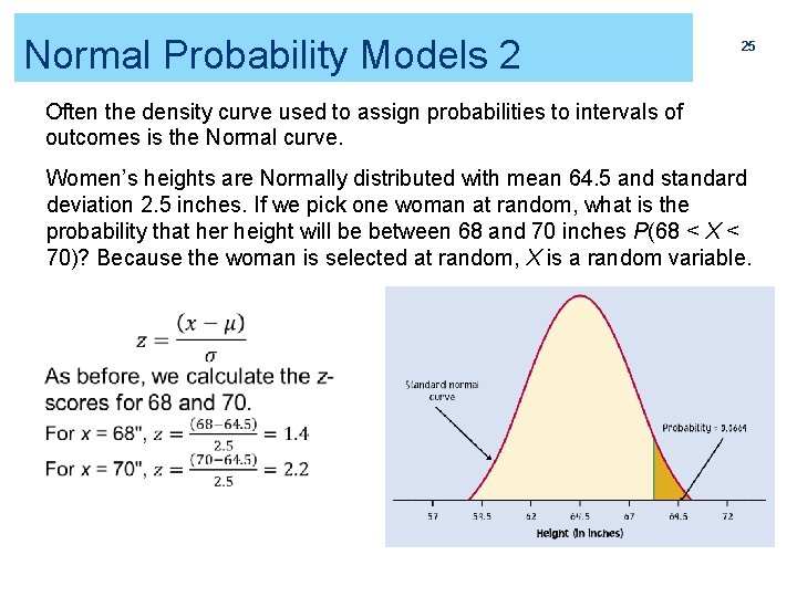
Normal Probability Models 2 25 Often the density curve used to assign probabilities to intervals of outcomes is the Normal curve. Women’s heights are Normally distributed with mean 64. 5 and standard deviation 2. 5 inches. If we pick one woman at random, what is the probability that her height will be between 68 and 70 inches P(68 < X < 70)? Because the woman is selected at random, X is a random variable.

4. 4 Means and Variances of Random Variables § The mean of a random variable § Statistical estimation and the law of large numbers § Rules for means § The variance of a random variable § Rules for variances and standard deviations 26

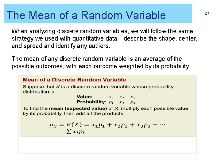
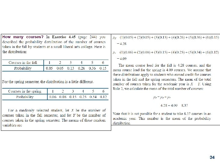
The Mean of a Random Variable When analyzing discrete random variables, we will follow the same strategy we used with quantitative data―describe the shape, center, and spread and identify any outliers. The mean of any discrete random variable is an average of the possible outcomes, with each outcome weighted by its probability. 27

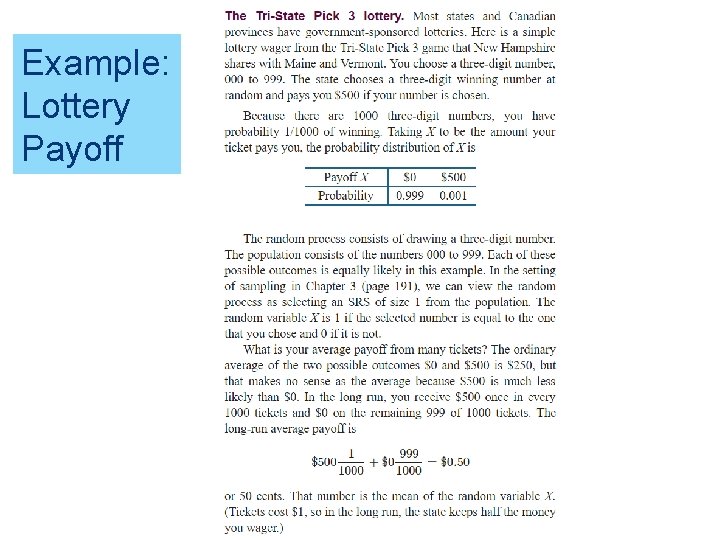
Example: Lottery Payoff

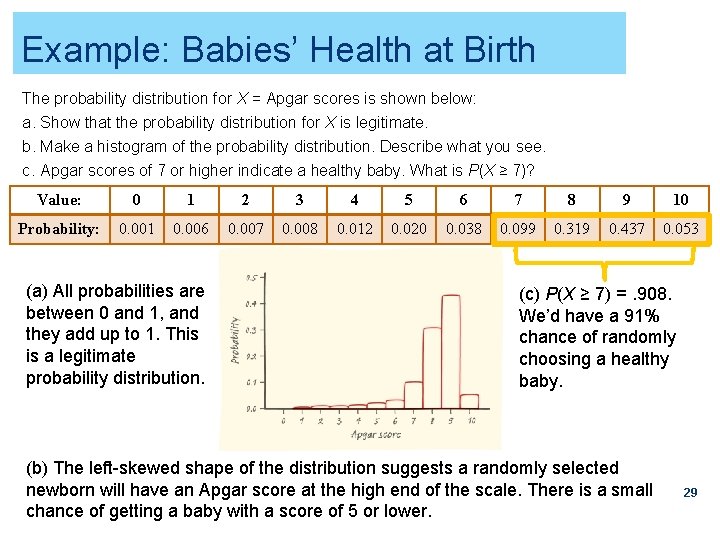
Example: Babies’ Health at Birth The probability distribution for X = Apgar scores is shown below: a. Show that the probability distribution for X is legitimate. b. Make a histogram of the probability distribution. Describe what you see. c. Apgar scores of 7 or higher indicate a healthy baby. What is P(X ≥ 7)? Value: 0 1 2 3 4 5 6 7 8 9 10 Probability: 0. 001 0. 006 0. 007 0. 008 0. 012 0. 020 0. 038 0. 099 0. 319 0. 437 0. 053 (a) All probabilities are between 0 and 1, and they add up to 1. This is a legitimate probability distribution. (c) P(X ≥ 7) =. 908. We’d have a 91% chance of randomly choosing a healthy baby. (b) The left-skewed shape of the distribution suggests a randomly selected newborn will have an Apgar score at the high end of the scale. There is a small chance of getting a baby with a score of 5 or lower. 29

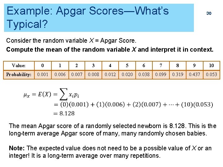
Example: Apgar Scores―What’s Typical? 30 Consider the random variable X = Apgar Score. Compute the mean of the random variable X and interpret it in context. Value: 0 1 2 3 4 5 6 7 8 9 10 Probability: 0. 001 0. 006 0. 007 0. 008 0. 012 0. 020 0. 038 0. 099 0. 319 0. 437 0. 053 The mean Apgar score of a randomly selected newborn is 8. 128. This is the long-term average Apgar score of many, many randomly chosen babies. Note: The expected value does not need to be a possible value of X or an integer! It is a long-term average over many repetitions.

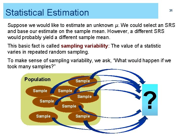
Statistical Estimation 31 Suppose we would like to estimate an unknown µ. We could select an SRS and base our estimate on the sample mean. However, a different SRS would probably yield a different sample mean. This basic fact is called sampling variability: The value of a statistic varies in repeated random sampling. To make sense of sampling variability, we ask, “What would happen if we took many samples? ” Population Sample Sample ?

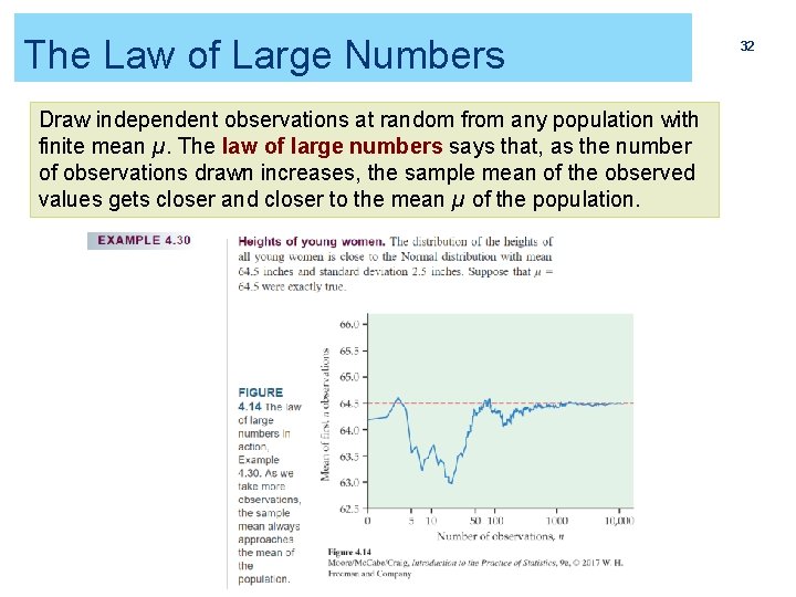
The Law of Large Numbers Draw independent observations at random from any population with finite mean µ. The law of large numbers says that, as the number of observations drawn increases, the sample mean of the observed values gets closer and closer to the mean µ of the population. 32

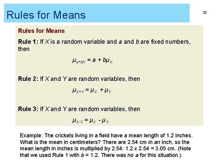
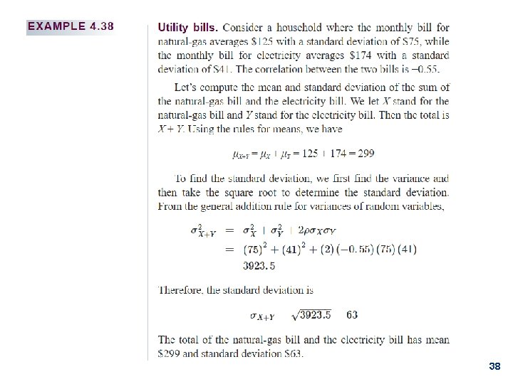
Rules for Means Rule 1: If X is a random variable and a and b are fixed numbers, then µa+b. X = a + bµX. Rule 2: If X and Y are random variables, then µX+Y = µX + µY. Rule 3: If X and Y are random variables, then µX-Y = µX - µY. Example: The crickets living in a field have a mean length of 1. 2 inches. What is the mean in centimeters? There are 2. 54 cm in an inch, so the mean length in inches is multiplied by 2. 54: 1. 2 x 2. 54 = 3. 05 cm. (Note that we used Rule 1 with b = 1. 2. There was no a for this situation. ) 33

34

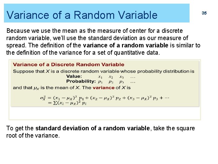
Variance of a Random Variable 35 Because we use the mean as the measure of center for a discrete random variable, we’ll use the standard deviation as our measure of spread. The definition of the variance of a random variable is similar to the definition of the variance for a set of quantitative data. To get the standard deviation of a random variable, take the square root of the variance.

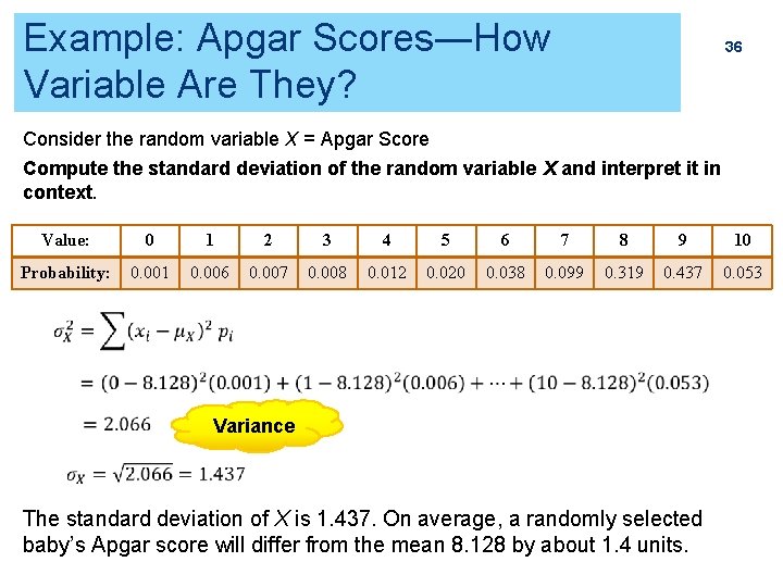
Example: Apgar Scores―How Variable Are They? 36 Consider the random variable X = Apgar Score Compute the standard deviation of the random variable X and interpret it in context. Value: 0 1 2 3 4 5 6 7 8 9 10 Probability: 0. 001 0. 006 0. 007 0. 008 0. 012 0. 020 0. 038 0. 099 0. 319 0. 437 0. 053 Variance The standard deviation of X is 1. 437. On average, a randomly selected baby’s Apgar score will differ from the mean 8. 128 by about 1. 4 units.

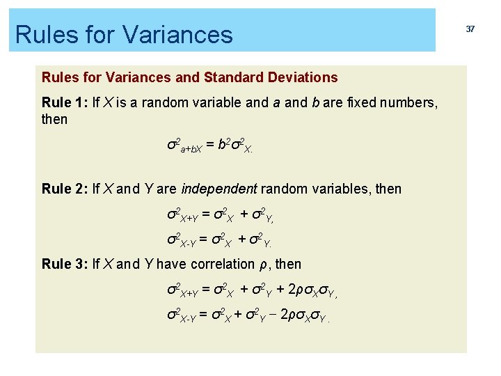
Rules for Variances and Standard Deviations Rule 1: If X is a random variable and a and b are fixed numbers, then σ2 a+b. X = b 2σ2 X. Rule 2: If X and Y are independent random variables, then σ2 X+Y = σ2 X + σ2 Y, σ2 X-Y = σ2 X + σ2 Y. Rule 3: If X and Y have correlation ρ, then σ2 X+Y = σ2 X + σ2 Y + 2ρσXσY , σ2 X-Y = σ2 X + σ2 Y 2ρσXσY. 37

38

4. 5 General Probability Rules* § Probability rules § General addition rules § Conditional probability § General multiplication rules § Tree diagrams § Bayes’s rule § Independence again 39

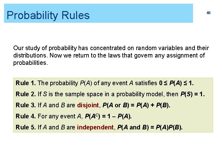
Probability Rules 40 Our study of probability has concentrated on random variables and their distributions. Now we return to the laws that govern any assignment of probabilities. Rule 1. The probability P(A) of any event A satisfies 0 ≤ P(A) ≤ 1. Rule 2. If S is the sample space in a probability model, then P(S) = 1. Rule 3. If A and B are disjoint, P(A or B) = P(A) + P(B). Rule 4. For any event A, P(AC) = 1 – P(A). Rule 5. If A and B are independent, P(A and B) = P(A)P(B).

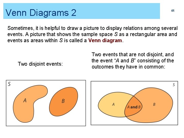
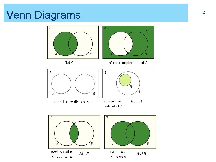
Venn Diagrams 2 41 Sometimes, it is helpful to draw a picture to display relations among several events. A picture that shows the sample space S as a rectangular area and events as areas within S is called a Venn diagram. Two disjoint events: Two events that are not disjoint, and the event “A and B” consisting of the outcomes they have in common:

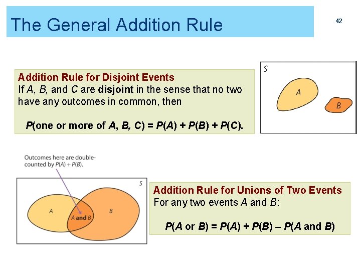
The General Addition Rule 42 Addition Rule for Disjoint Events If A, B, and C are disjoint in the sense that no two have any outcomes in common, then P(one or more of A, B, C) = P(A) + P(B) + P(C). Addition Rule for Unions of Two Events For any two events A and B: P(A or B) = P(A) + P(B) – P(A and B)

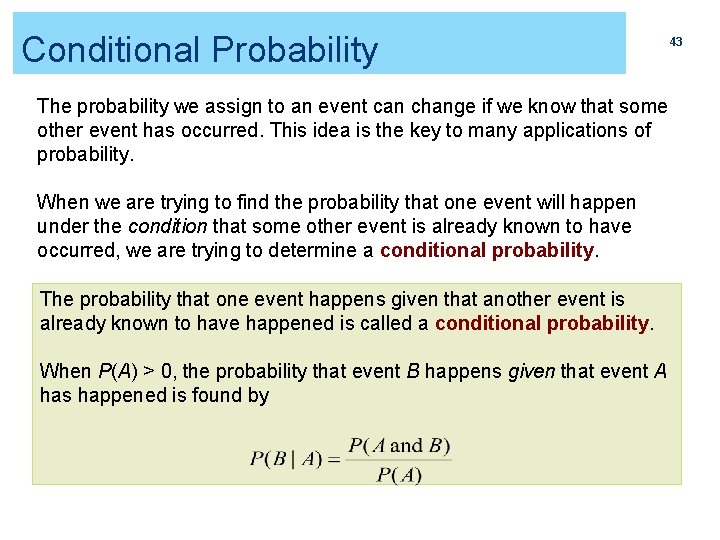
Conditional Probability 43 The probability we assign to an event can change if we know that some other event has occurred. This idea is the key to many applications of probability. When we are trying to find the probability that one event will happen under the condition that some other event is already known to have occurred, we are trying to determine a conditional probability. The probability that one event happens given that another event is already known to have happened is called a conditional probability. When P(A) > 0, the probability that event B happens given that event A has happened is found by

The General Multiplication Rule 44 The definition of conditional probability reminds us that, in principle, all probabilities, including conditional probabilities, can be found from the assignment of probabilities to events that describe a random phenomenon. The definition of conditional probability then turns into a rule for finding the probability that both of two events occur. The probability that events A and B both occur can be found using the general multiplication rule: P(A and B) = P(A) • P(B | A) where P(B | A) is the conditional probability that event B occurs given that event A has already occurred.

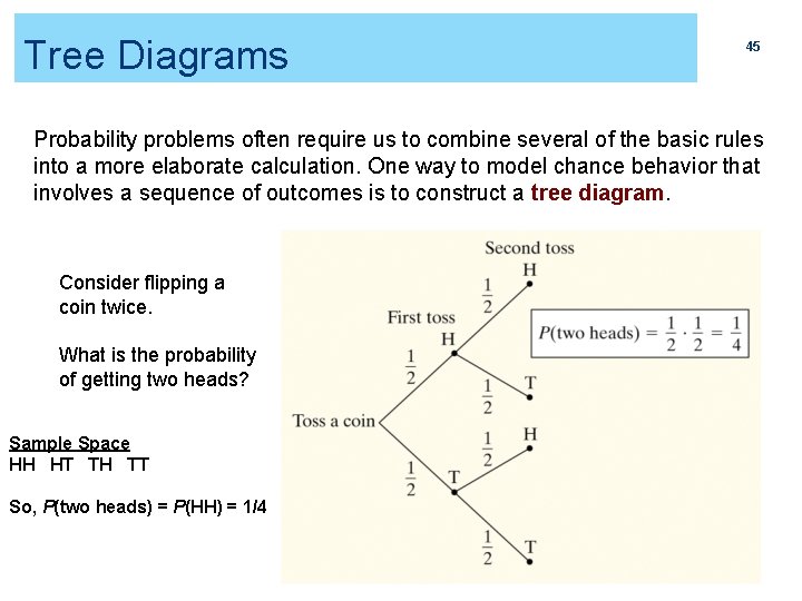
Tree Diagrams 45 Probability problems often require us to combine several of the basic rules into a more elaborate calculation. One way to model chance behavior that involves a sequence of outcomes is to construct a tree diagram. Consider flipping a coin twice. What is the probability of getting two heads? Sample Space HH HT TH TT So, P(two heads) = P(HH) = 1/4

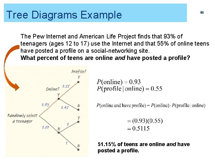
Tree Diagrams Example 46 The Pew Internet and American Life Project finds that 93% of teenagers (ages 12 to 17) use the Internet and that 55% of online teens have posted a profile on a social-networking site. What percent of teens are online and have posted a profile? 51. 15% of teens are online and have posted a profile.

Bayes’s Rule ¡ 47

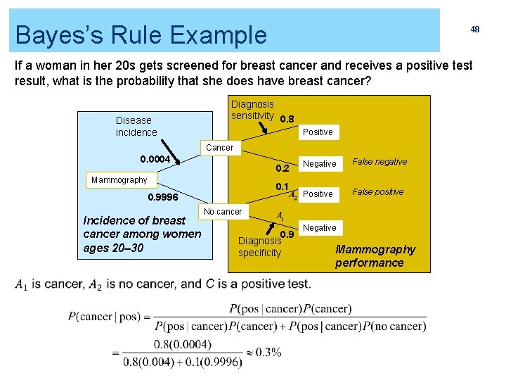
Bayes’s Rule Example 48 If a woman in her 20 s gets screened for breast cancer and receives a positive test result, what is the probability that she does have breast cancer? Disease incidence Diagnosis sensitivity 0. 8 Positive Cancer 0. 0004 0. 2 Mammography 0. 1 0. 9996 Incidence of breast cancer among women ages 20– 30 Negative False negative Positive False positive No cancer 0. 9 Diagnosis specificity Negative Mammography performance

Independence again 49 If two events A and B do not influence each other, and if knowledge about one does not change the probability of the other, the events are said to be independent of each other. Multiplication Rule for Independent Events Two events A and B are independent if knowing that one occurs does not change the probability that the other occurs. If A and B are independent: P(A and B) = P(A) P(B) Note: Two events A and B that both have positive probability are also independent if: P(B|A) = P(B)