Chapter 4 Partial Differential Equation PDE 1 Partial

Chapter 4 Partial Differential Equation (PDE) 1

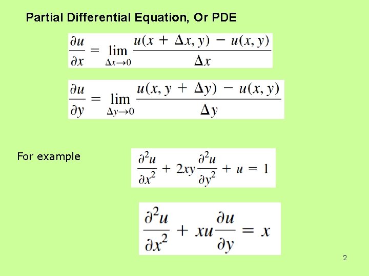
Partial Differential Equation, Or PDE For example 2

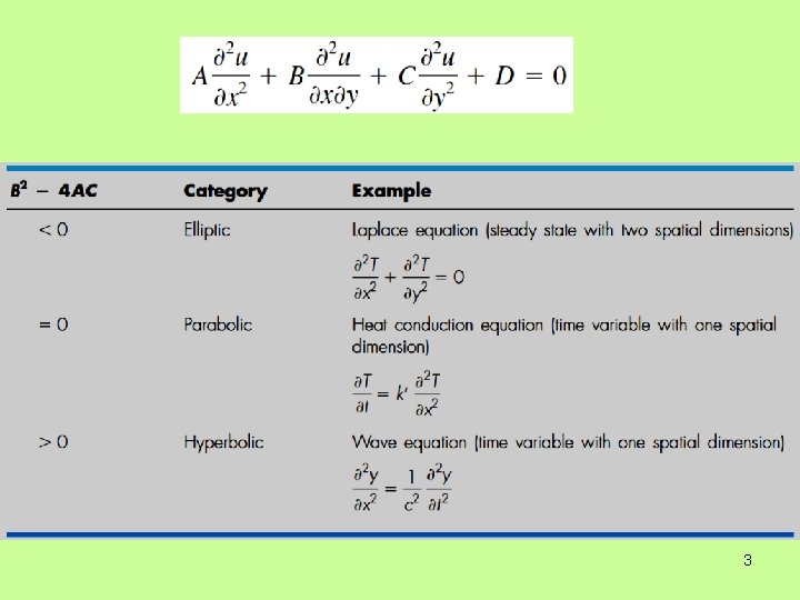
3

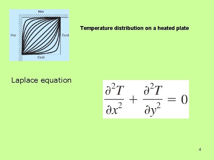
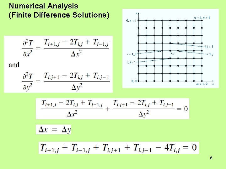
Temperature distribution on a heated plate Laplace equation 4

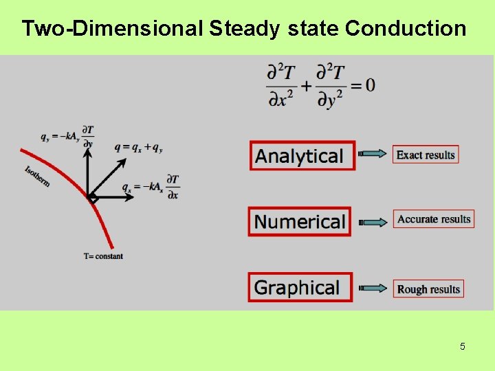
Two-Dimensional Steady state Conduction 5

Numerical Analysis (Finite Difference Solutions) 6

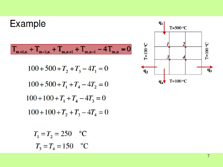
7

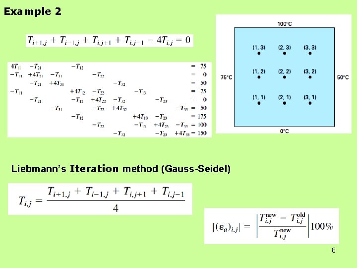
Example 2 Liebmann’s Iteration method (Gauss-Seidel) 8

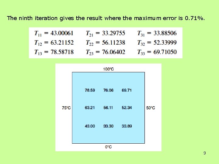
The ninth iteration gives the result where the maximum error is 0. 71%. 9

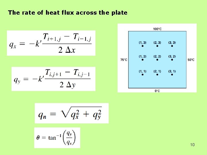
The rate of heat flux across the plate 10

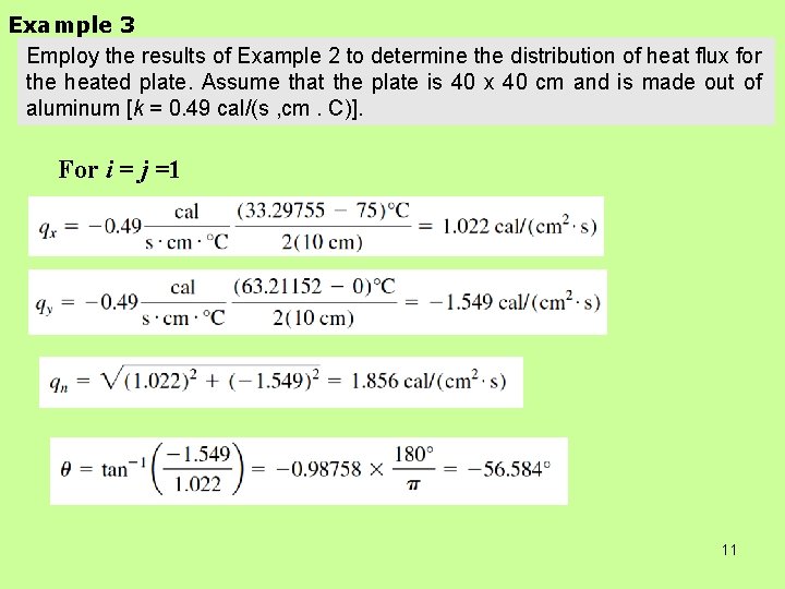
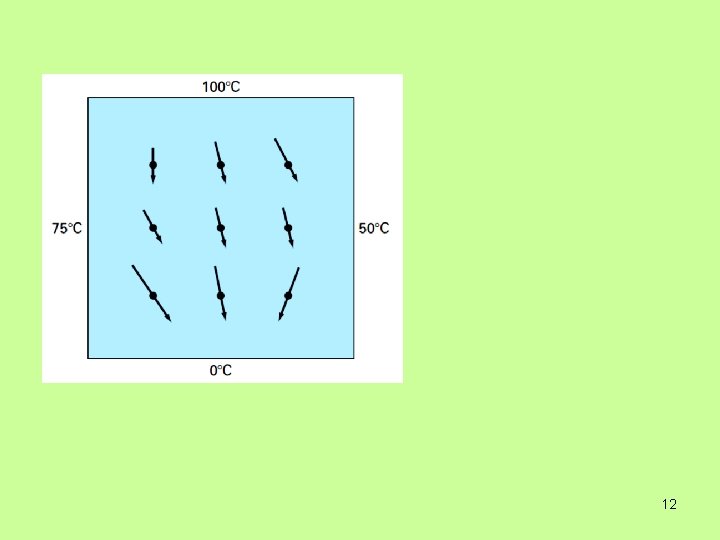
Example 3 Employ the results of Example 2 to determine the distribution of heat flux for the heated plate. Assume that the plate is 40 x 40 cm and is made out of aluminum [k = 0. 49 cal/(s , cm. C)]. For i = j =1 11

12

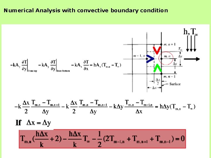
Numerical Analysis with convective boundary condition 13

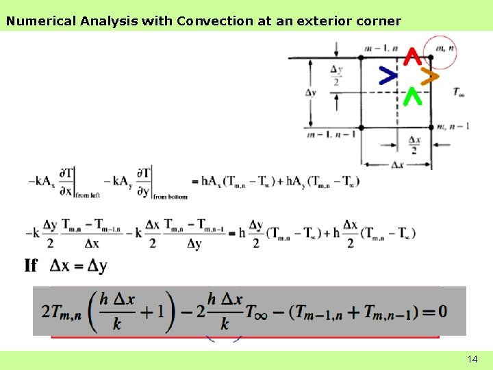
Numerical Analysis with Convection at an exterior corner 14

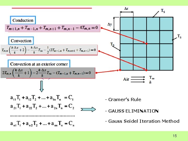
- Cramer’s Rule - GAUSS ELIMINATION - Gauss Seidel Iteration Method 15

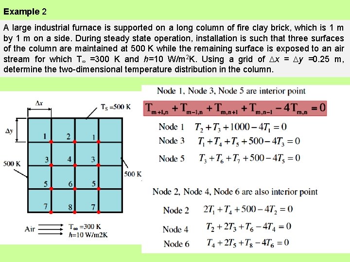
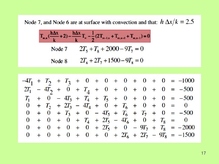
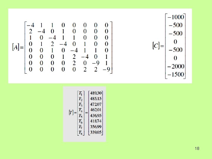
Example 2 A large industrial furnace is supported on a long column of fire clay brick, which is 1 m by 1 m on a side. During steady state operation, installation is such that three surfaces of the column are maintained at 500 K while the remaining surface is exposed to an air stream for which T∞ =300 K and h=10 W/m 2 K. Using a grid of Dx = Dy =0. 25 m, determine the two-dimensional temperature distribution in the column. 16

17

18

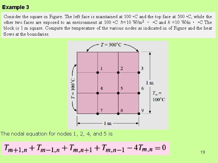
Example 3 Consider the square in Figure. The left face is maintained at 100 ◦C and the top face at 500 ◦C, while the other two faces are exposed to an environment at 100 ◦C: h=10 W/m 2 ・ ◦C and k =10 W/m・ ◦C The block is 1 m square. Compute the temperature of the various nodes as indicated in of Figure and the heat flows at the boundaries. The nodal equation for nodes 1, 2, 4, and 5 is 19

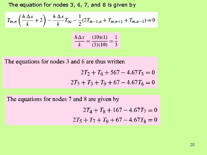
The equation for nodes 3, 6, 7, and 8 is given by 20

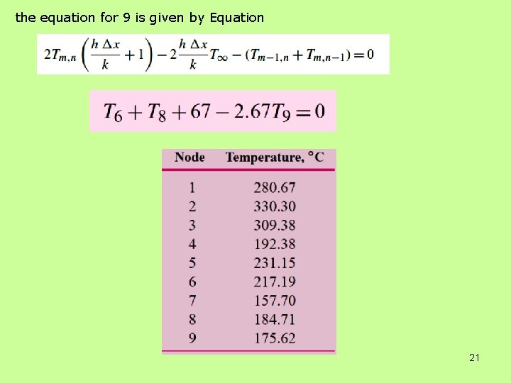
the equation for 9 is given by Equation 21

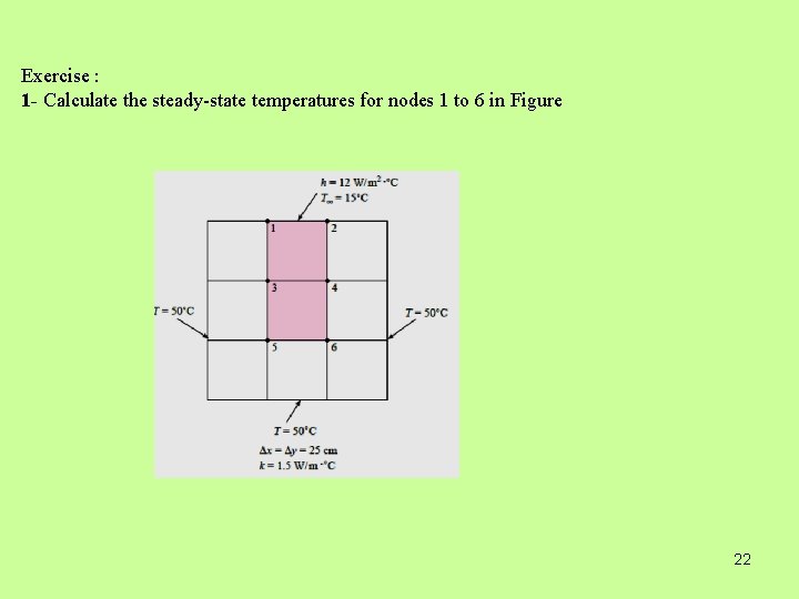
Exercise : 1 - Calculate the steady-state temperatures for nodes 1 to 6 in Figure 22

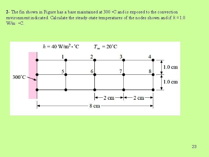
2 - The fin shown in Figure has a base maintained at 300 ◦C and is exposed to the convection environment indicated. Calculate the steady-state temperatures of the nodes shown and if k =1. 0 W/m· ◦C. 23