Chapter 4 Naive Approach Assumes demand in next

Chapter 4

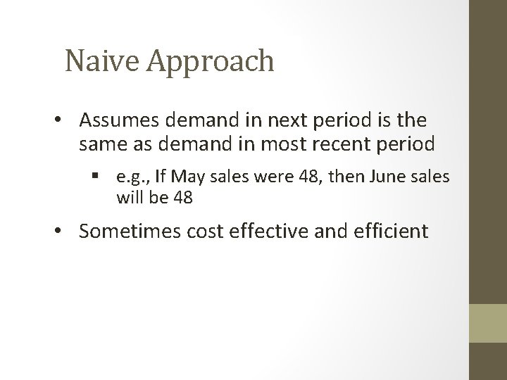
Naive Approach • Assumes demand in next period is the same as demand in most recent period § e. g. , If May sales were 48, then June sales will be 48 • Sometimes cost effective and efficient

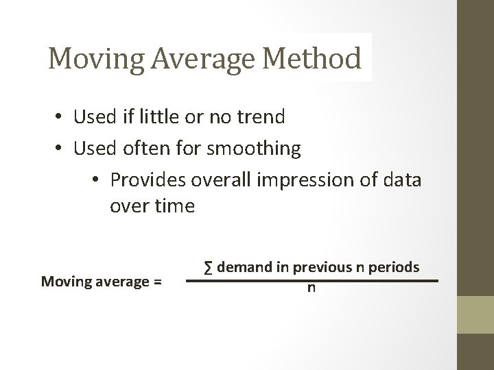
Moving Average Method • Used if little or no trend • Used often for smoothing • Provides overall impression of data over time Moving average = ∑ demand in previous n periods n

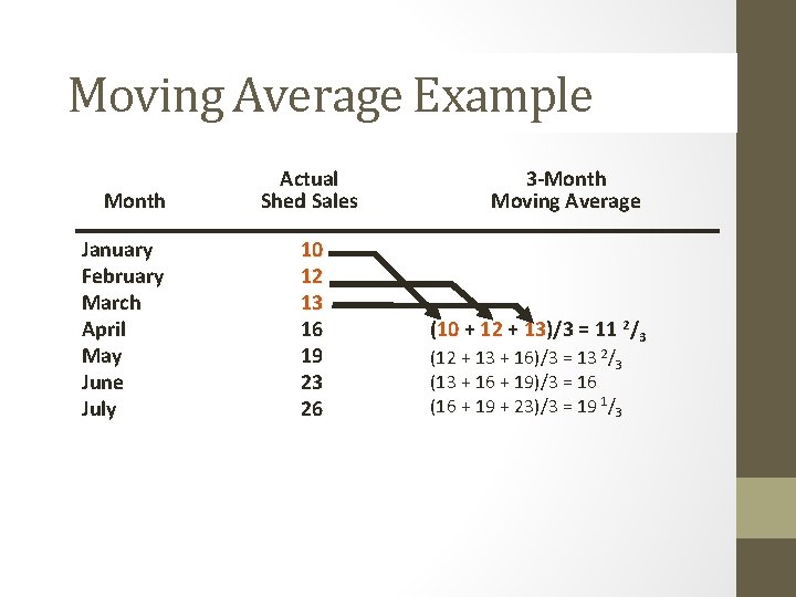
Moving Average Example Month January February March April May June July Actual Shed Sales 10 12 13 16 19 23 26 3 -Month Moving Average (10 + 12 + 13)/3 = 11 2/3 (12 + 13 + 16)/3 = 13 2/3 (13 + 16 + 19)/3 = 16 (16 + 19 + 23)/3 = 19 1/3

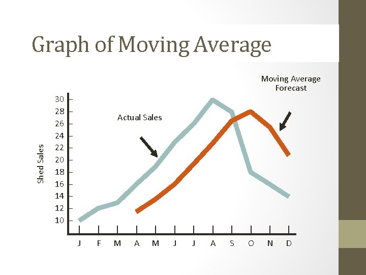
Shed Sales Graph of Moving Average 30 28 26 24 22 20 18 16 14 12 10 – – – Moving Average Forecast Actual Sales | J | F | M | A | M | J | A | S | O | N | D

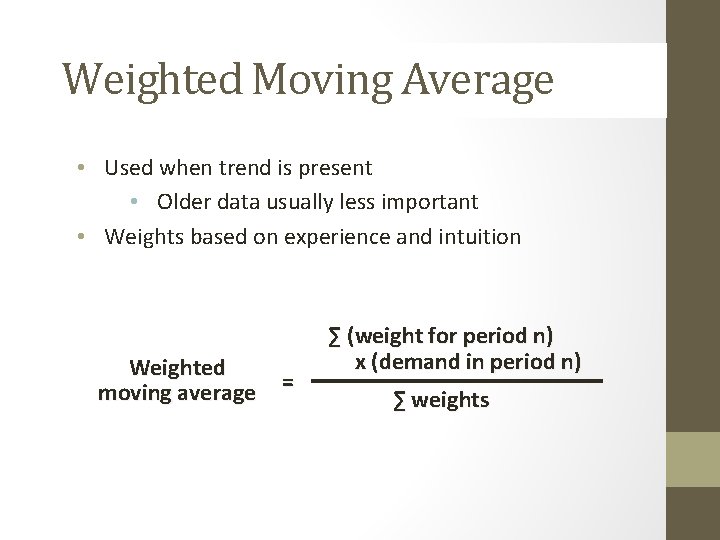
Weighted Moving Average • Used when trend is present • Older data usually less important • Weights based on experience and intuition Weighted moving average = ∑ (weight for period n) x (demand in period n) ∑ weights

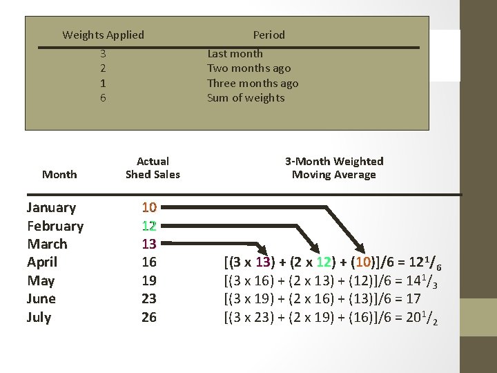
Weights Applied 3 2 1 6 Period Last month Two months ago Three months ago Sum of weights Weighted Moving Average Month January February March April May June July Actual Shed Sales 3 -Month Weighted Moving Average 10 12 13 16 19 23 26 [(3 x 13) + (2 x 12) + (10)]/6 = 121/6 [(3 x 16) + (2 x 13) + (12)]/6 = 141/3 [(3 x 19) + (2 x 16) + (13)]/6 = 17 [(3 x 23) + (2 x 19) + (16)]/6 = 201/2

Potential Problems With Moving Average • Increasing n smooths the forecast but makes it less sensitive to changes • Do not forecast trends well • Require extensive historical data

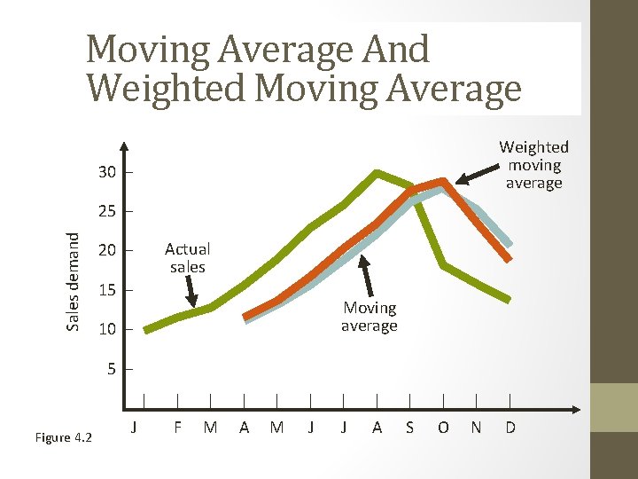
Moving Average And Weighted Moving Average Weighted moving average 30 – Sales demand 25 – Actual sales 20 – 15 – Moving average 10 – 5 – | Figure 4. 2 J | | | F M A M J J A S O N D

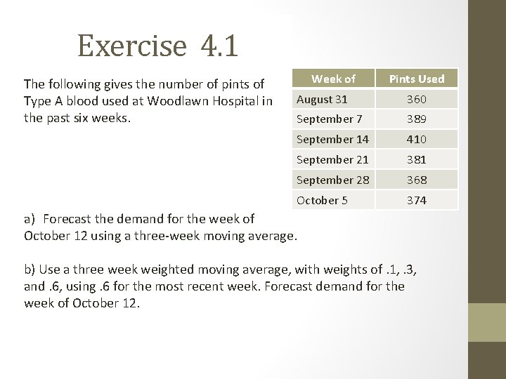
Exercise 4. 1 The following gives the number of pints of Type A blood used at Woodlawn Hospital in the past six weeks. Week of Pints Used August 31 360 September 7 389 September 14 410 September 21 381 September 28 368 October 5 374 a) Forecast the demand for the week of October 12 using a three-week moving average. b) Use a three week weighted moving average, with weights of. 1, . 3, and. 6, using. 6 for the most recent week. Forecast demand for the week of October 12.

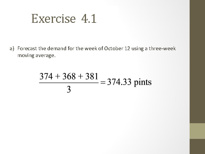
Exercise 4. 1 a) Forecast the demand for the week of October 12 using a three-week moving average.

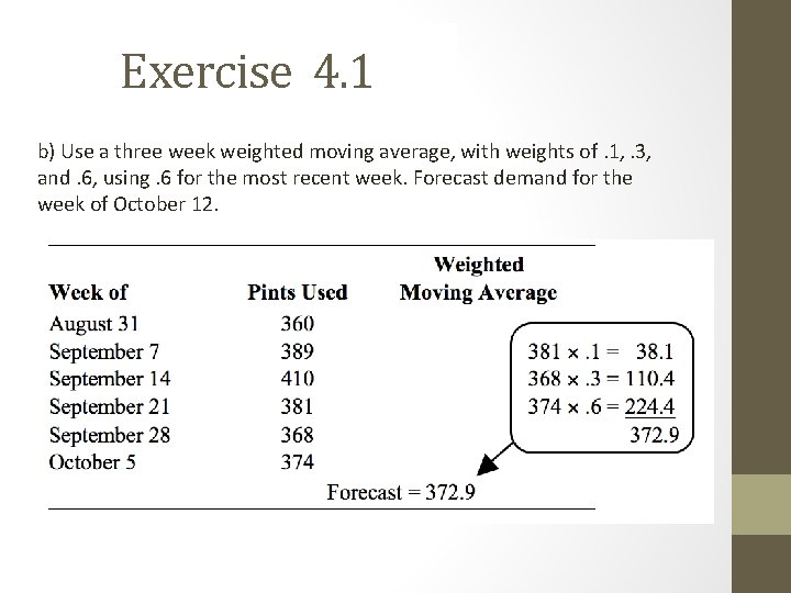
Exercise 4. 1 b) Use a three week weighted moving average, with weights of. 1, . 3, and. 6, using. 6 for the most recent week. Forecast demand for the week of October 12.