Chapter 4 Multiple Regression Analysis Copyright 2010 Pearson

Chapter 4 Multiple Regression Analysis Copyright © 2010 Pearson Education, Inc. , publishing as Prentice-Hall. 4 -1

Chapter 4 Multiple Regression Analysis LEARNING OBJECTIVES Upon completing this chapter, you should be able to do the following: • Determine when regression analysis is the appropriate statistical tool in analyzing a problem. • Understand how regression helps us make predictions using the least squares concept. • Use dummy variables with an understanding of their interpretation. • Be aware of the assumptions underlying regression analysis and how to assess them. Copyright © 2010 Pearson Education, Inc. , publishing as Prentice-Hall. 4 -2

Chapter 4 Multiple Regression Analysis LEARNING OBJECTIVES continued. . . Upon completing this chapter, you should be able to do the following: • Select an estimation technique and explain the difference between stepwise and simultaneous regression. • Interpret the results of regression. • Apply the diagnostic procedures necessary to assess “influential” observations. Copyright © 2010 Pearson Education, Inc. , publishing as Prentice-Hall. 4 -3

Multiple Regression Defined Multiple regression analysis. . . is a statistical technique that can be used to analyze the relationship between a single dependent (criterion) variable and several independent (predictor) variables. Copyright © 2010 Pearson Education, Inc. , publishing as Prentice-Hall. 4 -4

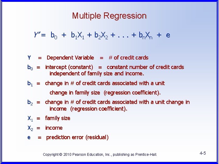
Multiple Regression Y’ = b 0 + b 1 X 1 + b 2 X 2 +. . . + bn. Xn + e Y = Dependent Variable = # of credit cards b 0 = intercept (constant) = constant number of credit cards independent of family size and income. b 1 = change in # of credit cards associated with a unit change in family size (regression coefficient). b 2 = change in # of credit cards associated with a unit change in income (regression coefficient). X 1 = family size X 2 = income e = prediction error (residual) Copyright © 2010 Pearson Education, Inc. , publishing as Prentice-Hall. 4 -5

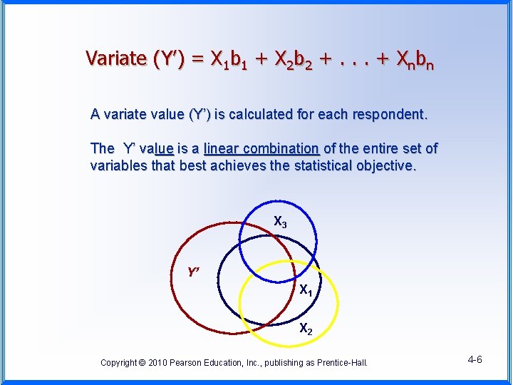
Variate (Y’) = X 1 b 1 + X 2 b 2 +. . . + Xnbn A variate value (Y’) is calculated for each respondent. The Y’ value is a linear combination of the entire set of variables that best achieves the statistical objective. X 3 Y’ X 1 X 2 Copyright © 2010 Pearson Education, Inc. , publishing as Prentice-Hall. 4 -6

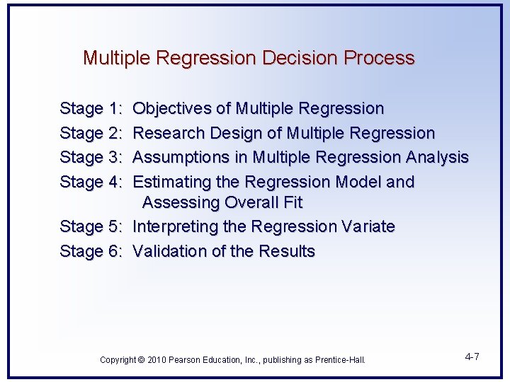
Multiple Regression Decision Process Stage 1: Stage 2: Stage 3: Stage 4: Objectives of Multiple Regression Research Design of Multiple Regression Assumptions in Multiple Regression Analysis Estimating the Regression Model and Assessing Overall Fit Stage 5: Interpreting the Regression Variate Stage 6: Validation of the Results Copyright © 2010 Pearson Education, Inc. , publishing as Prentice-Hall. 4 -7

Stage 1: Objectives of Multiple Regression In selecting suitable applications of multiple regression, the researcher must consider three primary issues: 1. 2. 3. the appropriateness of the research problem, specification of a statistical relationship, and selection of the dependent and independent variables. Copyright © 2010 Pearson Education, Inc. , publishing as Prentice-Hall. 4 -8

Selection of Dependent and Independent Variables The researcher should always consider three issues that can affect any decision about variables: • The theory that supports using the variables, • Measurement error, especially in the dependent variable, and • Specification error. Copyright © 2010 Pearson Education, Inc. , publishing as Prentice-Hall. 4 -9

Measurement Error in Regression Measurement error that is problematic can be addressed through either of two approaches: • Summated scales, or • Structural equation modeling procedures. Copyright © 2010 Pearson Education, Inc. , publishing as Prentice-Hall. 4 -10

Rules of Thumb 4– 1 Meeting Multiple Regression Objectives • Only structural equation modeling (SEM) can directly accommodate measurement error, but using summated scales can mitigate it when using multiple regression. • When in doubt, include potentially irrelevant variables (as they can only confuse interpretation) rather than possibly omitting a relevant variable (which can bias all regression estimates). Copyright © 2010 Pearson Education, Inc. , publishing as Prentice-Hall. 4 -11

Stage 2: Research Design of a Multiple Regression Analysis Issues to consider. . . • • Sample size, • Nature of independent variables – can be both fixed and random. Unique elements of the dependence relationship – can use dummy variables as independents, and Copyright © 2010 Pearson Education, Inc. , publishing as Prentice-Hall. 4 -12

Rules of Thumb 4– 2 Sample Size Considerations • Simple regression can be effective with a sample size of 20, but maintaining power at. 80 in multiple regression requires a minimum sample of 50 and preferably 100 observations for most research situations. • The minimum ratio of observations to variables is 5 to 1, but the preferred ratio is 15 or 20 to 1, and this should increase when stepwise estimation is used. • Maximizing the degrees of freedom improves generalizability and addresses both model parsimony and sample size concerns. Copyright © 2010 Pearson Education, Inc. , publishing as Prentice-Hall. 4 -13

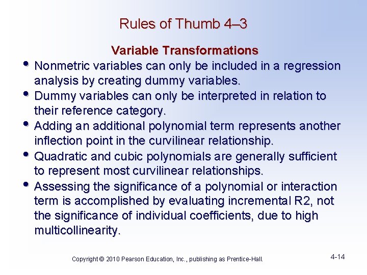
Rules of Thumb 4– 3 • • • Variable Transformations Nonmetric variables can only be included in a regression analysis by creating dummy variables. Dummy variables can only be interpreted in relation to their reference category. Adding an additional polynomial term represents another inflection point in the curvilinear relationship. Quadratic and cubic polynomials are generally sufficient to represent most curvilinear relationships. Assessing the significance of a polynomial or interaction term is accomplished by evaluating incremental R 2, not the significance of individual coefficients, due to high multicollinearity. Copyright © 2010 Pearson Education, Inc. , publishing as Prentice-Hall. 4 -14

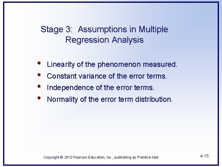
Stage 3: Assumptions in Multiple Regression Analysis • • Linearity of the phenomenon measured. Constant variance of the error terms. Independence of the error terms. Normality of the error term distribution. Copyright © 2010 Pearson Education, Inc. , publishing as Prentice-Hall. 4 -15

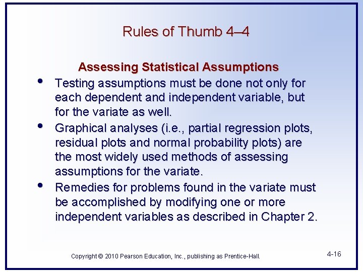
Rules of Thumb 4– 4 • • • Assessing Statistical Assumptions Testing assumptions must be done not only for each dependent and independent variable, but for the variate as well. Graphical analyses (i. e. , partial regression plots, residual plots and normal probability plots) are the most widely used methods of assessing assumptions for the variate. Remedies for problems found in the variate must be accomplished by modifying one or more independent variables as described in Chapter 2. Copyright © 2010 Pearson Education, Inc. , publishing as Prentice-Hall. 4 -16

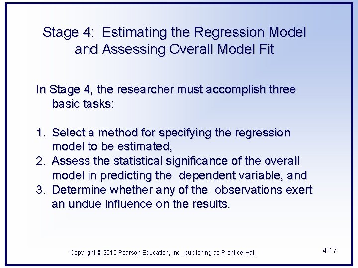
Stage 4: Estimating the Regression Model and Assessing Overall Model Fit In Stage 4, the researcher must accomplish three basic tasks: 1. Select a method for specifying the regression model to be estimated, 2. Assess the statistical significance of the overall model in predicting the dependent variable, and 3. Determine whether any of the observations exert an undue influence on the results. Copyright © 2010 Pearson Education, Inc. , publishing as Prentice-Hall. 4 -17

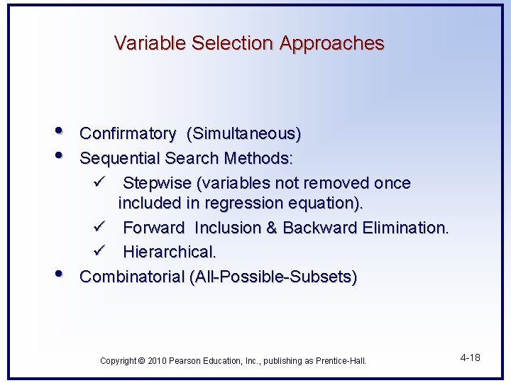
Variable Selection Approaches • • • Confirmatory (Simultaneous) Sequential Search Methods: ü Stepwise (variables not removed once included in regression equation). ü Forward Inclusion & Backward Elimination. ü Hierarchical. Combinatorial (All-Possible-Subsets) Copyright © 2010 Pearson Education, Inc. , publishing as Prentice-Hall. 4 -18

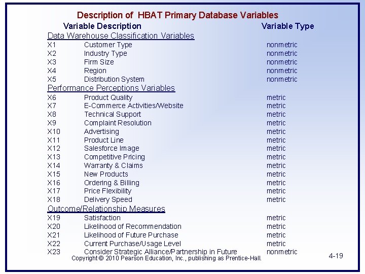
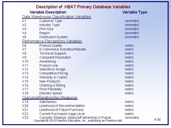
Description of HBAT Primary Database Variables Variable Description Data Warehouse Classification Variables X 1 X 2 X 3 X 4 X 5 Variable Type Customer Type Industry Type Firm Size Region Distribution System nonmetric nonmetric Performance Perceptions Variables X 6 X 7 X 8 X 9 X 10 X 11 X 12 X 13 X 14 X 15 X 16 X 17 X 18 Product Quality E-Commerce Activities/Website Technical Support Complaint Resolution Advertising Product Line Salesforce Image Competitive Pricing Warranty & Claims New Products Ordering & Billing Price Flexibility Delivery Speed metric metric metric metric Outcome/Relationship Measures X 19 X 20 X 21 X 22 X 23 Satisfaction Likelihood of Recommendation Likelihood of Future Purchase Current Purchase/Usage Level Consider Strategic Alliance/Partnership in Future Copyright © 2010 Pearson Education, Inc. , publishing as Prentice-Hall. metric nonmetric 4 -19

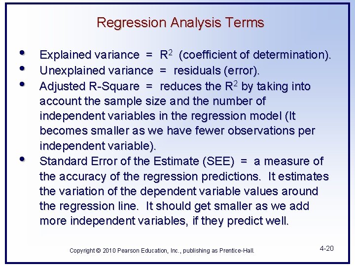
Regression Analysis Terms • • Explained variance = R 2 (coefficient of determination). Unexplained variance = residuals (error). Adjusted R-Square = reduces the R 2 by taking into account the sample size and the number of independent variables in the regression model (It becomes smaller as we have fewer observations per independent variable). Standard Error of the Estimate (SEE) = a measure of the accuracy of the regression predictions. It estimates the variation of the dependent variable values around the regression line. It should get smaller as we add more independent variables, if they predict well. Copyright © 2010 Pearson Education, Inc. , publishing as Prentice-Hall. 4 -20

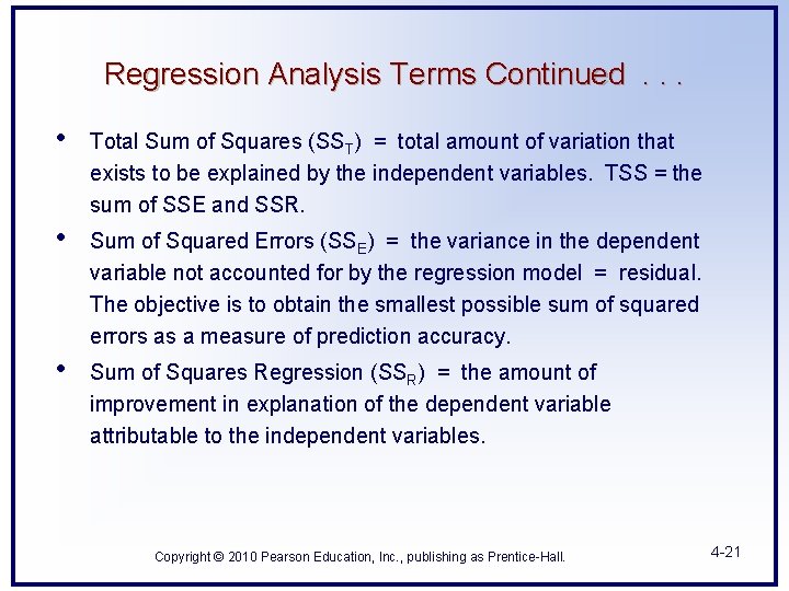
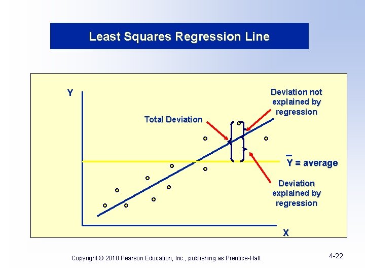
Regression Analysis Terms Continued. . . • Total Sum of Squares (SST) = total amount of variation that exists to be explained by the independent variables. TSS = the sum of SSE and SSR. • Sum of Squared Errors (SSE) = the variance in the dependent variable not accounted for by the regression model = residual. The objective is to obtain the smallest possible sum of squared errors as a measure of prediction accuracy. • Sum of Squares Regression (SSR) = the amount of improvement in explanation of the dependent variable attributable to the independent variables. Copyright © 2010 Pearson Education, Inc. , publishing as Prentice-Hall. 4 -21

Least Squares Regression Line Y Total Deviation not explained by regression Y = average Deviation explained by regression X Copyright © 2010 Pearson Education, Inc. , publishing as Prentice-Hall. 4 -22

Statistical vs. Practical Significance? The F statistic is used to determine if the overall regression model is statistically significant. If the F statistic is significant, it means it is unlikely your sample will produce a large R 2 when the population R 2 is actually zero. To be considered statistically significant, a rule of thumb is there must be <. 05 probability the results are due to chance. If the R 2 is statistically significant, we then evaluate the strength of the linear association between the dependent variable and the several independent variables. R 2, also called the coefficient of determination, is used to measure the strength of the overall relationship. It represents the amount of variation in the dependent variable associated with all of the independent variables considered together (it also is referred to as a measure of the goodness of fit). R 2 ranges from 0 to 1. 0 and represents the amount of the dependent variable “explained” by the independent variables combined. A large R 2 indicates the straight line works well while a small R 2 indicates it does not work well. Even though an R 2 is statistically significant, it does not mean it is practically significant. We also must ask whether the results are meaningful. For example, is the value of knowing you have explained 4 percent of the variation worth the cost of collecting and analyzing the data? Copyright © 2010 Pearson Education, Inc. , publishing as Prentice-Hall. 4 -23

Rules of Thumb 4– 5 • • Estimation Techniques No matter which estimation technique is chosen, theory must be a guiding factor in evaluating the final regression model because: ü Confirmatory Specification, the only method to allow direct testing of a prespecified model, is also the most complex from the perspectives of specification error, model parsimony and achieving maximum predictive accuracy. ü Sequential search (e. g. , stepwise), while maximizing predictive accuracy, represents a completely “automated” approach to model estimation, leaving the researcher almost no control over the final model specification. ü Combinatorial estimation, while considering all possible models, still removes control from the researcher in terms of final model specification even though the researcher can view the set of roughly equivalent models in terms of predictive accuracy. No single method is “Best” and the prudent strategy is to use a combination of approaches to capitalize on the strengths of each to reflect theoretical basis of the research question. Copyright © 2010 Pearson Education, Inc. , publishing as Prentice-Hall. 4 -24

Regression Coefficient Questions Three questions about the statistical significance of any regression coefficient: 1) Was statistical significance established? 2) How does the sample size come into play? 3) Does it have practical significance in addition to statistical significance? Copyright © 2010 Pearson Education, Inc. , publishing as Prentice-Hall. 4 -25

Rules of Thumb 4– 6 • • Statistical Significance and Influential Observations Always ensure practical significance when using large sample sizes, as the model results and regression coefficients could be deemed irrelevant even when statistically significant due just to the statistical power arising from large sample sizes. Use the adjusted R 2 as your measure of overall model predictive accuracy. Statistical significance is required for a relationship to have validity, but statistical significance without theoretical support does not support validity. While outliers may be easily identifiable, the other forms of influential observations requiring more specialized diagnostic methods can be equal to or even more impactful on the results. Copyright © 2010 Pearson Education, Inc. , publishing as Prentice-Hall. 4 -26

Types of Influential Observations Influential observations. . . include all observations that have a disproportionate effect on the regression results. There are three basic types based upon the nature of their impact on the regression results: • • • Outliers are observations that have large residual values and can be identified only with respect to a specific regression model. Leverage points are observations that are distinct from the remaining observations based on their independent variable values. Influential observations are the broadest category, including all observations that have a disproportionate effect on the regression results. Influential observations potentially include outliers and leverage points but may include other observations as well. Copyright © 2010 Pearson Education, Inc. , publishing as Prentice-Hall. 4 -27

Corrective Actions for Influentials 1. 2. 3. 4. Influentials, outliers, and leverage points are based on one of four conditions, each of which has a specific course of corrective action: An error in observations or data entry – remedy by correcting the data or deleting the case, A valid but exceptional observation that is explainable by an extraordinary situation – remedy by deletion of the case unless variables reflecting the extraordinary situation are included in the regression equation, An exceptional observation with no likely explanation – presents a special problem because there is no reason for deleting the case, but its inclusion cannot be justified either, suggesting analyses with and without the observations to make a complete assessment, and An ordinary observation in its individual characteristics but exceptional in its combination of characteristics – indicates modifications to the conceptual basis of the regression model and should be retained. Copyright © 2010 Pearson Education, Inc. , publishing as Prentice-Hall. 4 -28

Assessing Multicollinearity The researcher’s task is to. . . • Assess the degree of multicollinearity, • Determine its impact on the results, and • Apply the necessary remedies if needed. Copyright © 2010 Pearson Education, Inc. , publishing as Prentice-Hall. 4 -29

Multicollinearity Diagnostics • Variance Inflation Factor (VIF) – measures how much the variance of the regression coefficients is inflated by multicollinearity problems. If VIF equals 0, there is no correlation between the independent measures. A VIF measure of 1 is an indication of some association between predictor variables, but generally not enough to cause problems. A maximum acceptable VIF value would be 10; anything higher would indicate a problem with multicollinearity. • Tolerance – the amount of variance in an independent variable that is not explained by the other independent variables. If the other variables explain a lot of the variance of a particular independent variable we have a problem with multicollinearity. Thus, small values for tolerance indicate problems of multicollinearity. The minimum cutoff value for tolerance is typically. 10. That is, the tolerance value must be smaller than. 10 to indicate a problem of multicollinearity. Copyright © 2010 Pearson Education, Inc. , publishing as Prentice-Hall. 4 -30

Interpretation of Regression Results • • Coefficient of Determination Regression Coefficients (Unstandardized – bivariate) • • • Beta Coefficients (Standardized) Variables Entered Multicollinearity ? ? Copyright © 2010 Pearson Education, Inc. , publishing as Prentice-Hall. 4 -31

Rules of Thumb 4– 7 • • Interpreting the Regression Variate Interpret the impact of each independent variable relative to the other variables in the model, as model respecification can have a profound effect on the remaining variables: ü Use beta weights when comparing relative importance among independent variables. ü Regression coefficients describe changes in the dependent variable, but can be difficult in comparing across independent variables if the response formats vary. Multicollinearity may be considered “good” when it reveals a suppressor effect, but generally it is viewed as harmful since increases in multicollinearity: ü reduce the overall R 2 that can be achieved, ü confound estimation of the regression coefficients, and ü negatively affect the statistical significance tests of coefficients. Copyright © 2010 Pearson Education, Inc. , publishing as Prentice-Hall. 4 -32

Rules of Thumb 4– 7 continued. . . Interpreting the Regression Variate • Generally accepted levels of multicollinearity (tolerance values up to. 10, corresponding to a VIF of 10) almost always indicate problems with multicollinearity, but these problems may be seen at much lower levels of collinearity or multicollinearity. ü Bivariate correlations of. 70 or higher may result in problems, and even lower correlations may be problematic if they are higher than the correlations between the dependent and independent variables. ü Values much lower than the suggested thresholds (VIF values of even 3 to 5) may result in interpretation or estimation problems, particularly when the relationships with the dependent variable are weaker. Copyright © 2010 Pearson Education, Inc. , publishing as Prentice-Hall. 4 -33

Residuals Plots • Histogram of standardized residuals – enables you to determine if the errors are normally distributed. • Normal probability plot – enables you to determine if the errors are normally distributed. It compares the observed (sample) standardized residuals against the expected standardized residuals from a normal distribution. • Scatter. Plot of residuals – can be used to test regression assumptions. It compares the standardized predicted values of the dependent variable against the standardized residuals from the regression equation. If the plot exhibits a random pattern then this indicates no identifiable violations of the assumptions underlying regression analysis. Copyright © 2010 Pearson Education, Inc. , publishing as Prentice-Hall. 4 -34

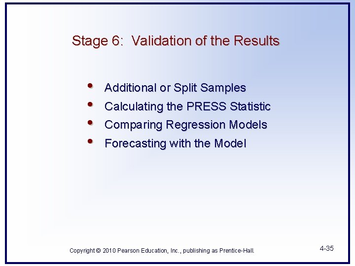
Stage 6: Validation of the Results • • Additional or Split Samples Calculating the PRESS Statistic Comparing Regression Models Forecasting with the Model Copyright © 2010 Pearson Education, Inc. , publishing as Prentice-Hall. 4 -35

Description of HBAT Primary Database Variables Variable Description Data Warehouse Classification Variables X 1 X 2 X 3 X 4 X 5 Variable Type Customer Type Industry Type Firm Size Region Distribution System nonmetric nonmetric Performance Perceptions Variables X 6 X 7 X 8 X 9 X 10 X 11 X 12 X 13 X 14 X 15 X 16 X 17 X 18 Product Quality E-Commerce Activities/Website Technical Support Complaint Resolution Advertising Product Line Salesforce Image Competitive Pricing Warranty & Claims New Products Ordering & Billing Price Flexibility Delivery Speed metric metric metric metric Outcome/Relationship Measures X 19 X 20 X 21 X 22 X 23 Satisfaction Likelihood of Recommendation Likelihood of Future Purchase Current Purchase/Usage Level Consider Strategic Alliance/Partnership in Future Copyright © 2010 Pearson Education, Inc. , publishing as Prentice-Hall. metric nonmetric 4 -36

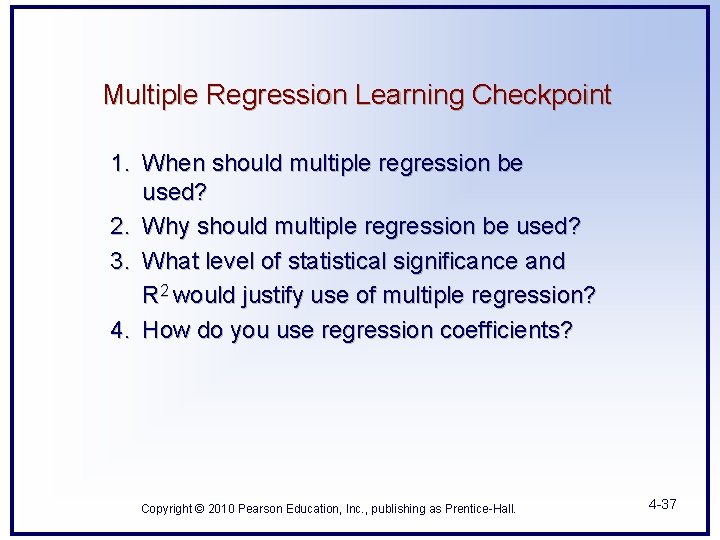
Multiple Regression Learning Checkpoint 1. When should multiple regression be used? 2. Why should multiple regression be used? 3. What level of statistical significance and R 2 would justify use of multiple regression? 4. How do you use regression coefficients? Copyright © 2010 Pearson Education, Inc. , publishing as Prentice-Hall. 4 -37