Chapter 4 Multilayer Percetrons Neural Networks Simon Haykin

Chapter - 4 Multilayer Percetrons Neural Networks, Simon Haykin, Prentice-Hall, 2 nd edition

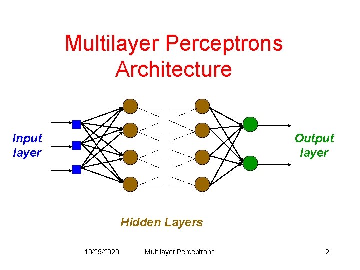
Multilayer Perceptrons Architecture Input layer Output layer Hidden Layers 10/29/2020 Multilayer Perceptrons 2

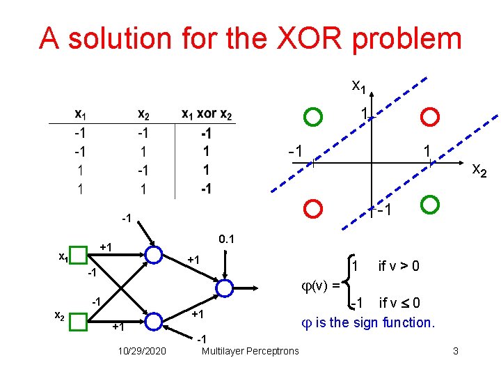
A solution for the XOR problem x 1 1 -1 -1 0. 1 +1 x 1 +1 -1 (v) = -1 x 2 +1 +1 10/29/2020 -1 Multilayer Perceptrons 1 if v > 0 -1 if v 0 is the sign function. 3

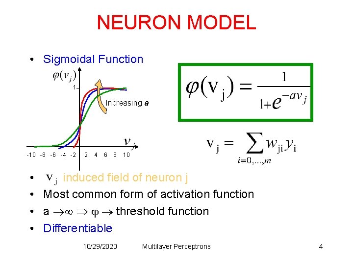
NEURON MODEL • Sigmoidal Function 1 Increasing a -10 -8 -6 -4 -2 2 4 6 8 10 • induced field of neuron j • Most common form of activation function • a threshold function • Differentiable 10/29/2020 Multilayer Perceptrons 4

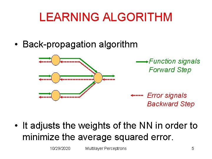
LEARNING ALGORITHM • Back-propagation algorithm Function signals Forward Step Error signals Backward Step • It adjusts the weights of the NN in order to minimize the average squared error. 10/29/2020 Multilayer Perceptrons 5

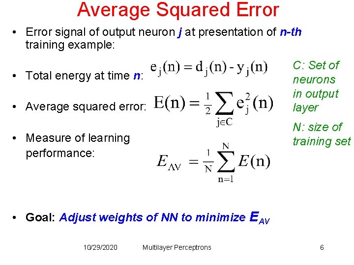
Average Squared Error • Error signal of output neuron j at presentation of n-th training example: • Total energy at time n: • Average squared error: C: Set of neurons in output layer N: size of training set • Measure of learning performance: • Goal: Adjust weights of NN to minimize EAV 10/29/2020 Multilayer Perceptrons 6

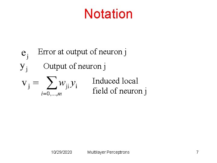
Notation Error at output of neuron j Output of neuron j Induced local field of neuron j 10/29/2020 Multilayer Perceptrons 7

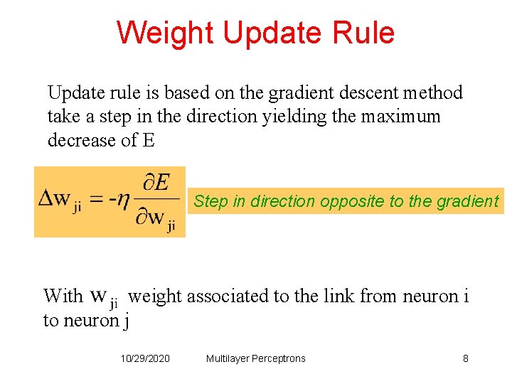
Weight Update Rule Update rule is based on the gradient descent method take a step in the direction yielding the maximum decrease of E Step in direction opposite to the gradient With weight associated to the link from neuron i to neuron j 10/29/2020 Multilayer Perceptrons 8

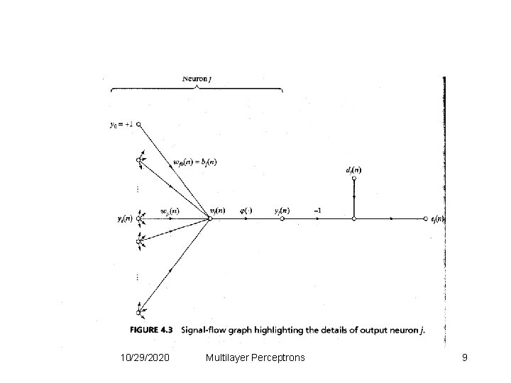
10/29/2020 Multilayer Perceptrons 9

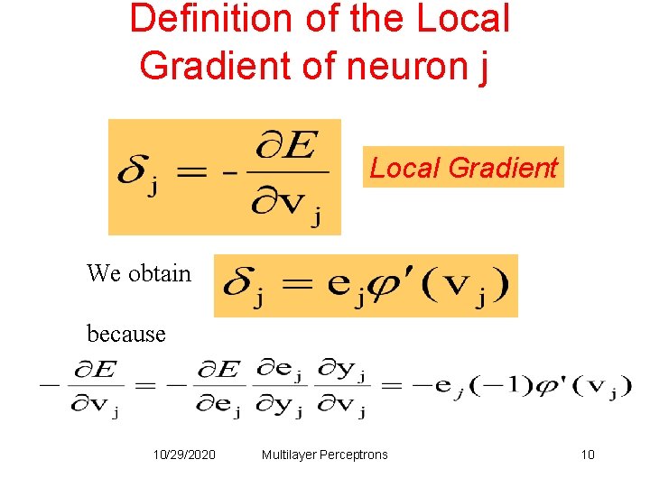
Definition of the Local Gradient of neuron j Local Gradient We obtain because 10/29/2020 Multilayer Perceptrons 10

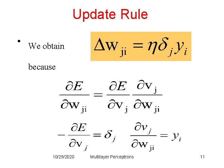
Update Rule • We obtain because 10/29/2020 Multilayer Perceptrons 11

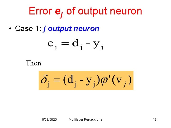
Compute local gradient of neuron j • The key factor is the calculation of ej • There are two cases: – Case 1): j is a output neuron – Case 2): j is a hidden neuron 10/29/2020 Multilayer Perceptrons 12

Error ej of output neuron • Case 1: j output neuron Then 10/29/2020 Multilayer Perceptrons 13

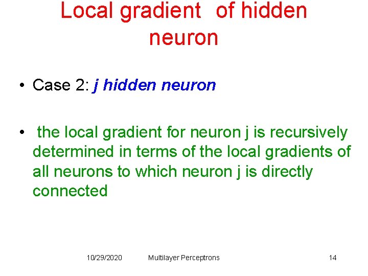
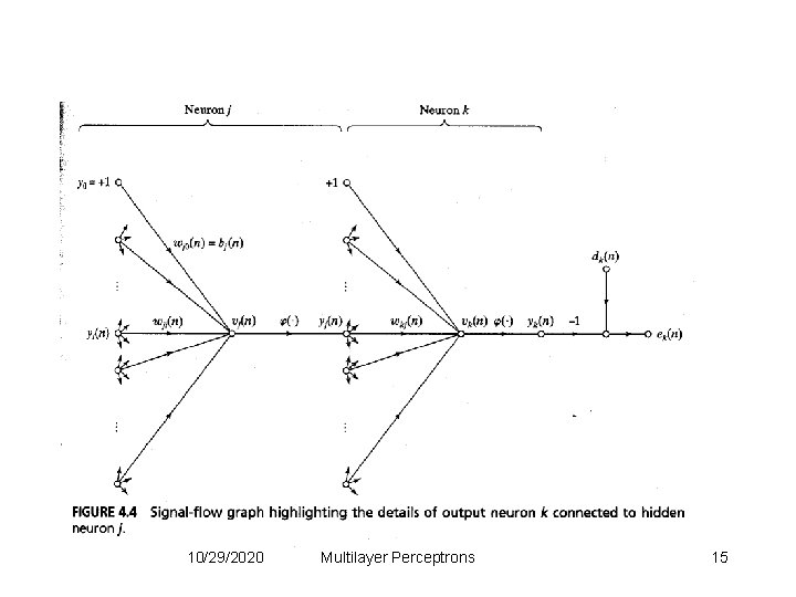
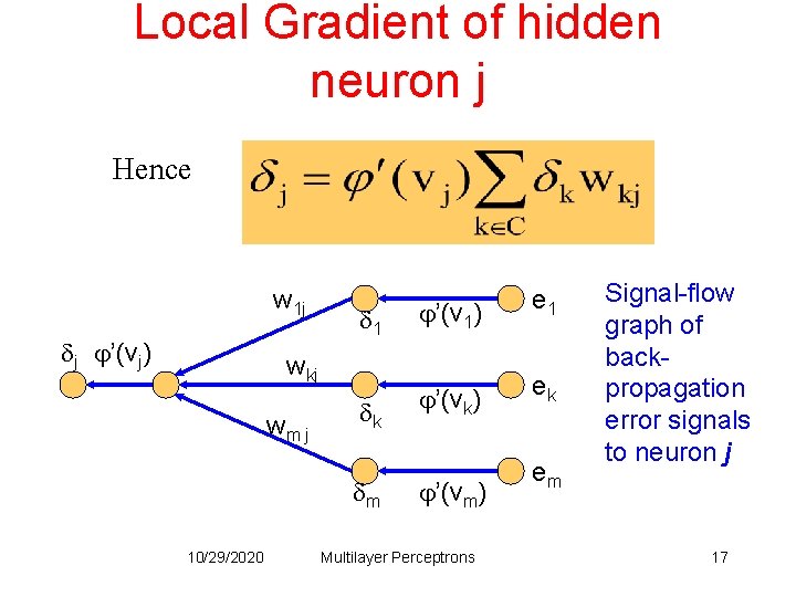
Local gradient of hidden neuron • Case 2: j hidden neuron • the local gradient for neuron j is recursively determined in terms of the local gradients of all neurons to which neuron j is directly connected 10/29/2020 Multilayer Perceptrons 14

10/29/2020 Multilayer Perceptrons 15

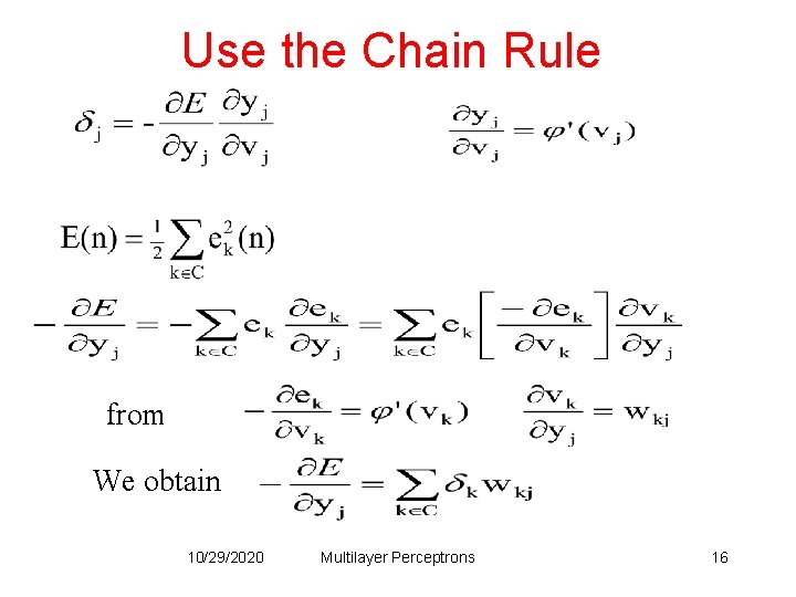
Use the Chain Rule from We obtain 10/29/2020 Multilayer Perceptrons 16

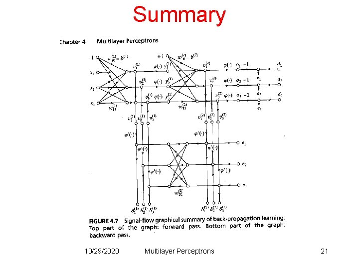
Local Gradient of hidden neuron j Hence w 1 j j ’(vj) 1 wkj wm j k m 10/29/2020 ’(v 1) e 1 ’(vk) ek ’(vm) Multilayer Perceptrons em Signal-flow graph of backpropagation error signals to neuron j 17

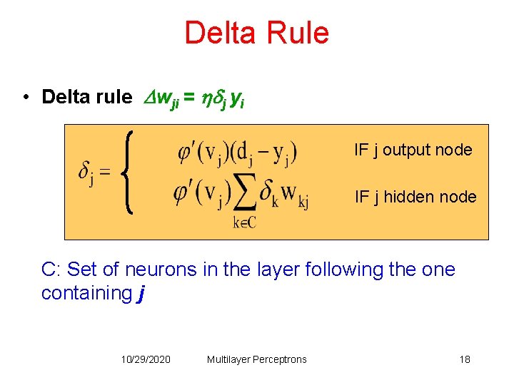
Delta Rule • Delta rule wji = j yi IF j output node IF j hidden node C: Set of neurons in the layer following the one containing j 10/29/2020 Multilayer Perceptrons 18

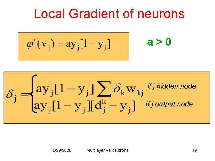
Local Gradient of neurons a>0 if j hidden node If j output node 10/29/2020 Multilayer Perceptrons 19

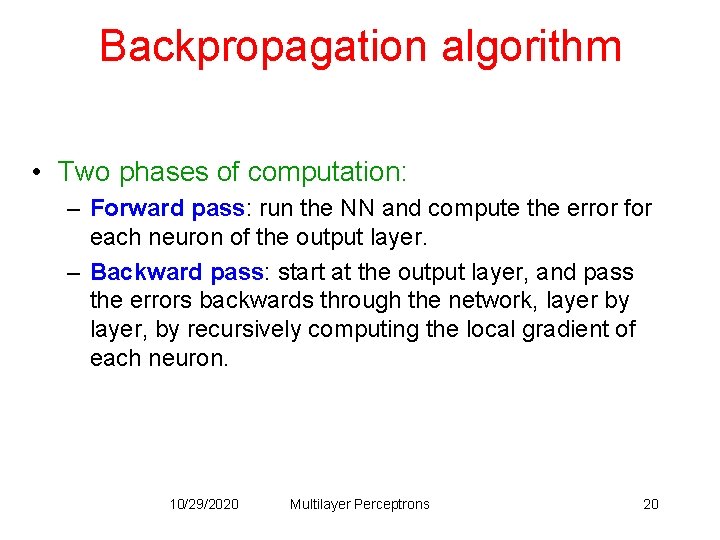
Backpropagation algorithm • Two phases of computation: – Forward pass: run the NN and compute the error for each neuron of the output layer. – Backward pass: start at the output layer, and pass the errors backwards through the network, layer by layer, by recursively computing the local gradient of each neuron. 10/29/2020 Multilayer Perceptrons 20

Summary 10/29/2020 Multilayer Perceptrons 21

Training • Sequential mode (on-line, pattern or stochastic mode): – (x(1), d(1)) is presented, a sequence of forward and backward computations is performed, and the weights are updated using the delta rule. – Same for (x(2), d(2)), … , (x(N), d(N)). 10/29/2020 Multilayer Perceptrons 22

Training • The learning process continues on an epoch-by -epoch basis until the stopping condition is satisfied. • From one epoch to the next choose a randomized ordering for selecting examples in the training set. 10/29/2020 Multilayer Perceptrons 23

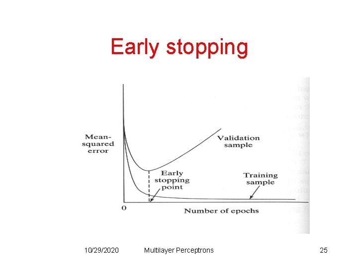
Stopping criterions • Sensible stopping criterions: – Average squared error change: Back-prop is considered to have converged when the absolute rate of change in the average squared error per epoch is sufficiently small (in the range [0. 1, 0. 01]). – Generalization based criterion: After each epoch the NN is tested for generalization. If the generalization performance is adequate then stop. 10/29/2020 Multilayer Perceptrons 24

Early stopping 10/29/2020 Multilayer Perceptrons 25

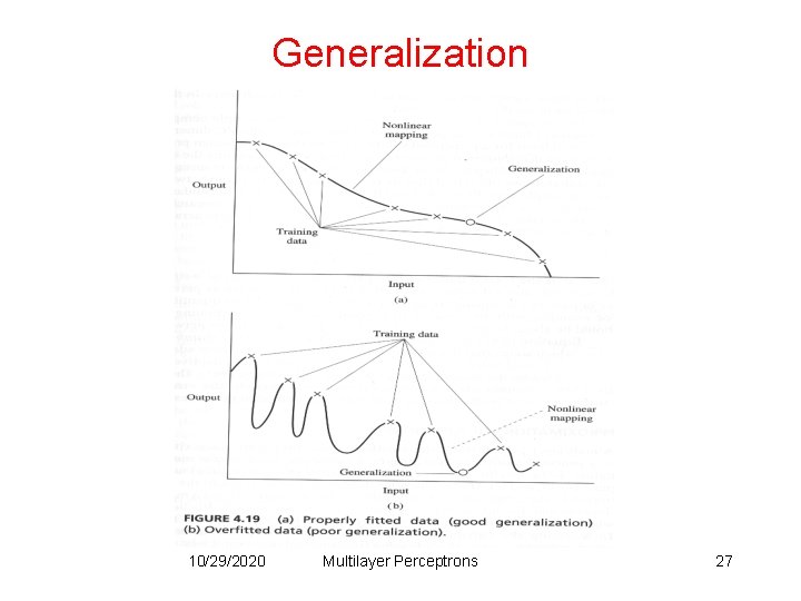
Generalization • Generalization: NN generalizes well if the I/O mapping computed by the network is nearly correct for new data (test set). • Factors that influence generalization: – the size of the training set. – the architecture of the NN. – the complexity of the problem at hand. • Overfitting (overtraining): when the NN learns too many I/O examples it may end up memorizing the training data. 10/29/2020 Multilayer Perceptrons 26

Generalization 10/29/2020 Multilayer Perceptrons 27

Expressive capabilities of NN Boolean functions: • Every boolean function can be represented by network with single hidden layer • but might require exponential hidden units Continuous functions: • Every bounded continuous function can be approximated with arbitrarily small error, by network with one hidden layer • Any function can be approximated with arbitrary accuracy by a network with two hidden layers 10/29/2020 Multilayer Perceptrons 28

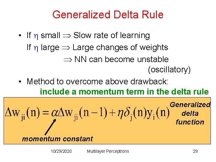
Generalized Delta Rule • If small Slow rate of learning If large Large changes of weights NN can become unstable (oscillatory) • Method to overcome above drawback: include a momentum term in the delta rule Generalized delta function momentum constant 10/29/2020 Multilayer Perceptrons 29

Generalized delta rule • the momentum accelerates the descent in steady downhill directions. • the momentum has a stabilizing effect in directions that oscillate in time. 10/29/2020 Multilayer Perceptrons 30

adaptation Heuristics for accelerating the convergence of the back-prop algorithm through adaptation: • Heuristic 1: Every weight should have its own . • Heuristic 2: Every should be allowed to vary from one iteration to the next. 10/29/2020 Multilayer Perceptrons 31

NN DESIGN • • • Data representation Network Topology Network Parameters Training Validation 10/29/2020 Multilayer Perceptrons 32

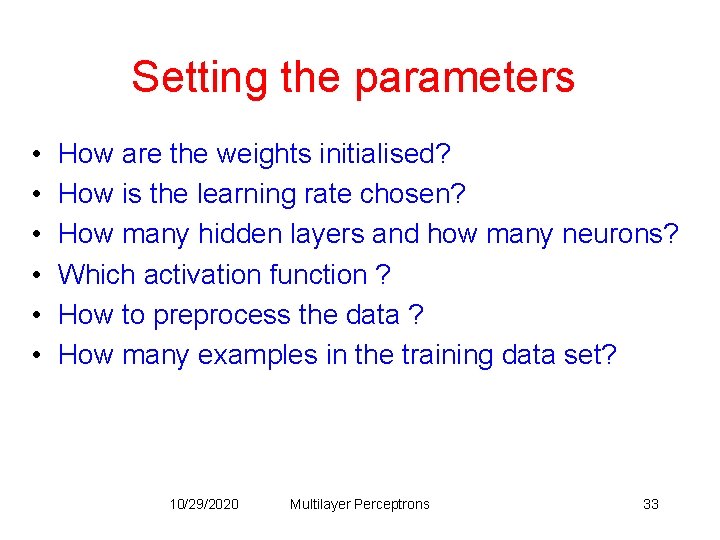
Setting the parameters • • • How are the weights initialised? How is the learning rate chosen? How many hidden layers and how many neurons? Which activation function ? How to preprocess the data ? How many examples in the training data set? 10/29/2020 Multilayer Perceptrons 33

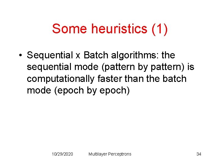
Some heuristics (1) • Sequential x Batch algorithms: the sequential mode (pattern by pattern) is computationally faster than the batch mode (epoch by epoch) 10/29/2020 Multilayer Perceptrons 34

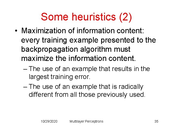
Some heuristics (2) • Maximization of information content: every training example presented to the backpropagation algorithm must maximize the information content. – The use of an example that results in the largest training error. – The use of an example that is radically different from all those previously used. 10/29/2020 Multilayer Perceptrons 35

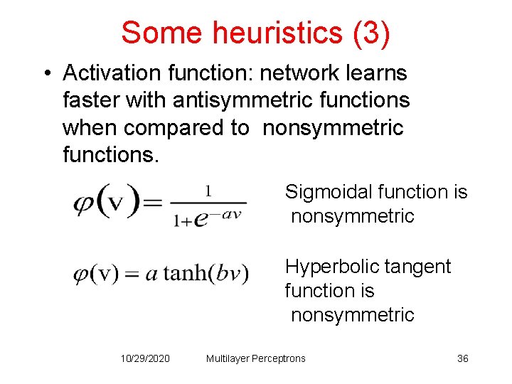
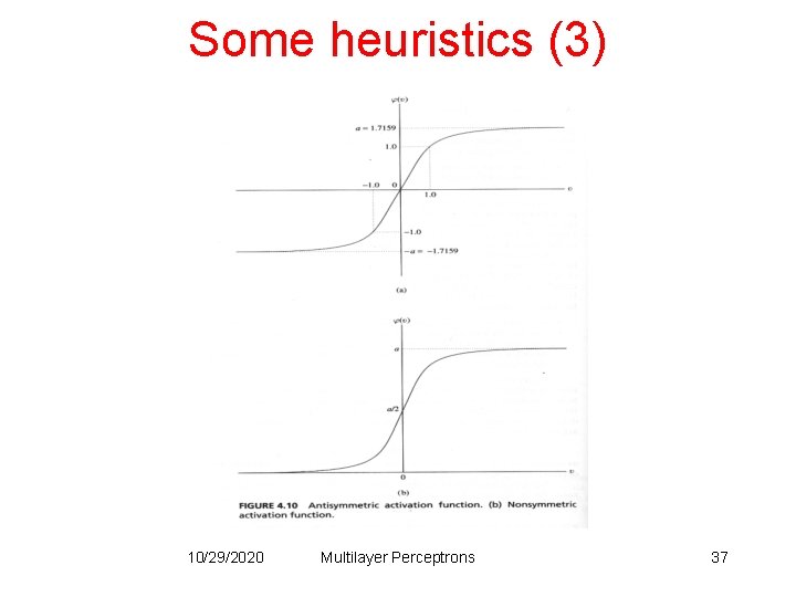
Some heuristics (3) • Activation function: network learns faster with antisymmetric functions when compared to nonsymmetric functions. Sigmoidal function is nonsymmetric Hyperbolic tangent function is nonsymmetric 10/29/2020 Multilayer Perceptrons 36

Some heuristics (3) 10/29/2020 Multilayer Perceptrons 37

Some heuristics (4) • Target values: target values must be chosen within the range of the sigmoidal activation function. • Otherwise, hidden neurons can be driven into saturation which slows down learning 10/29/2020 Multilayer Perceptrons 38

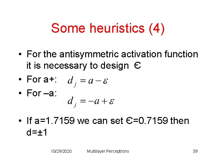
Some heuristics (4) • For the antisymmetric activation function it is necessary to design Є • For a+: • For –a: • If a=1. 7159 we can set Є=0. 7159 then d=± 1 10/29/2020 Multilayer Perceptrons 39

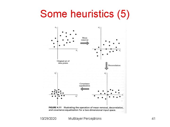
Some heuristics (5) • Inputs normalisation: – Each input variable should be processed so that the mean value is small or close to zero or at least very small when compared to the standard deviation. – Input variables should be uncorrelated. – Decorrelated input variables should be scaled so their covariances are approximately equal. 10/29/2020 Multilayer Perceptrons 40

Some heuristics (5) 10/29/2020 Multilayer Perceptrons 41

Some heuristics (6) • Initialisation of weights: – If synaptic weights are assigned large initial values neurons are driven into saturation. Local gradients become small so learning rate becomes small. – If synaptic weights are assigned small initial values algorithms operate around the origin. For the hyperbolic activation function the origin is a saddle point. 10/29/2020 Multilayer Perceptrons 42

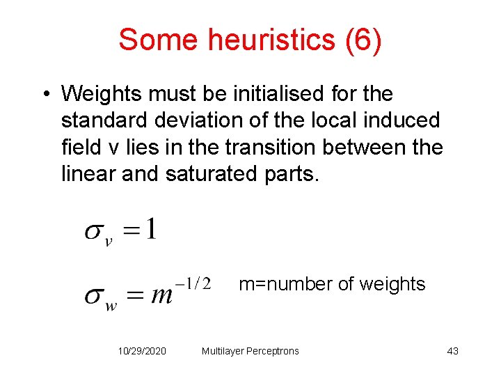
Some heuristics (6) • Weights must be initialised for the standard deviation of the local induced field v lies in the transition between the linear and saturated parts. m=number of weights 10/29/2020 Multilayer Perceptrons 43

Some heuristics (7) • Learning rate: – The right value of depends on the application. Values between 0. 1 and 0. 9 have been used in many applications. – Other heuristics adapt during the training as described in previous slides. 10/29/2020 Multilayer Perceptrons 44

Some heuristics (8) • How many layers and neurons – The number of layers and of neurons depend on the specific task. In practice this issue is solved by trial and error. – Two types of adaptive algorithms can be used: • start from a large network and successively remove some neurons and links until network performance degrades. • begin with a small network and introduce new neurons until performance is satisfactory. 10/29/2020 Multilayer Perceptrons 45

Some heuristics (9) • How many training data ? – Rule of thumb: the number of training examples should be at least five to ten times the number of weights of the network. 10/29/2020 Multilayer Perceptrons 46

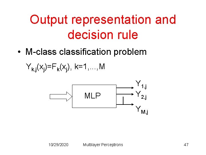
Output representation and decision rule • M-classification problem Yk, j(xj)=Fk(xj), k=1, . . . , M MLP Y 1, j Y 2, j YM, j 10/29/2020 Multilayer Perceptrons 47

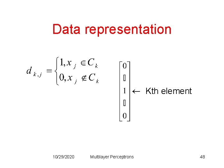
Data representation Kth element 10/29/2020 Multilayer Perceptrons 48

MLP and the a posteriori class probability • A multilayer perceptron classifier (using the logistic function) aproximate the a posteriori class probabilities, provided that the size of the training set is large enough. 10/29/2020 Multilayer Perceptrons 49

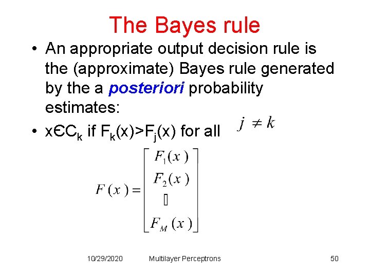
The Bayes rule • An appropriate output decision rule is the (approximate) Bayes rule generated by the a posteriori probability estimates: • xЄCk if Fk(x)>Fj(x) for all 10/29/2020 Multilayer Perceptrons 50