Chapter 4 Minitab Summarising bivariate data Correlation coefficient

Chapter 4 Minitab: Summarising bivariate data

Correlation coefficient • Enter the data from Example 4. 1 in columns C 1 and C 2 of the worksheet.

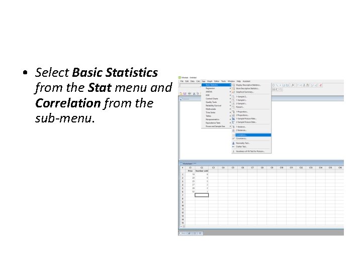
• Select Basic Statistics from the Stat menu and Correlation from the sub-menu.

• Type C 1 and C 2 in the space under Variables. • Click OK.

• The correlation coefficient appears in the session window.

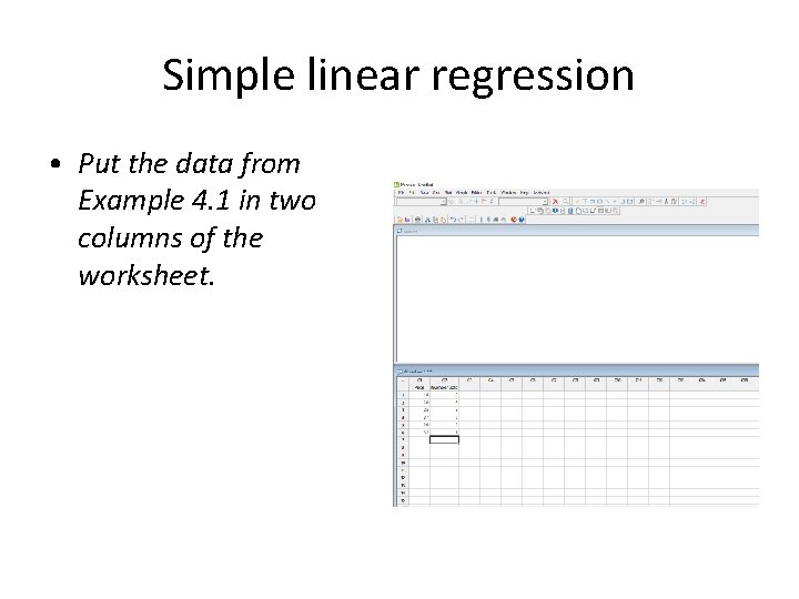
Simple linear regression • Put the data from Example 4. 1 in two columns of the worksheet.

• Select Regression from the Stat menu then Regression from the Regression sub-menu then Fit Regression Model from the next menu.

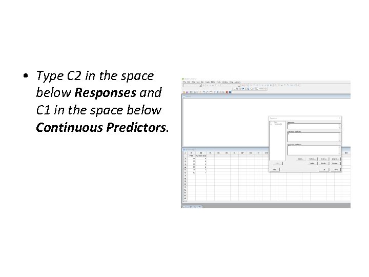
• Type C 2 in the space below Responses and C 1 in the space below Continuous Predictors.

• Click OK and the output that appears has the regression equation, the equation of the line of best fit, at the bottom.

• For a scatter diagram with the line of best-fit superimposed on the scatter like Figure 4. 11 follow the Stat – Regression sequence and choose Fitted Line Plot from the Regression sub-menu.

• Type C 2 beside Response (Y) and C 1 beside Predictor (X). • Click OK.

• The diagram that appears includes the regression equation and the value of R 2 for the data.

Time series decomposition • Put the data from Example 4. 12 into C 1 in chronological order.

• Select Time Series from the Stat menu then Decomposition from the sub-menu.

• Type C 1 to the right of Variable, type 3 as the Seasonal length and select the Additive model under Model Type. • Click OK.

• The output generated includes three graphs, the third of which is a plot of the series with the trend estimates.