Chapter 4 Linear Programming The Simplex Method n

Chapter 4 Linear Programming: The Simplex Method n n n n An Overview of the Simplex Method Standard Form Tableau Form Setting Up the Initial Simplex Tableau Improving the Solution Calculating the Next Tableau Solving a Minimization Problem Special Cases 1

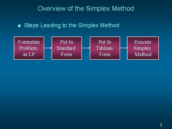
Overview of the Simplex Method n Steps Leading to the Simplex Method Formulate Problem as LP Put In Standard Form Put In Tableau Form Execute Simplex Method 2

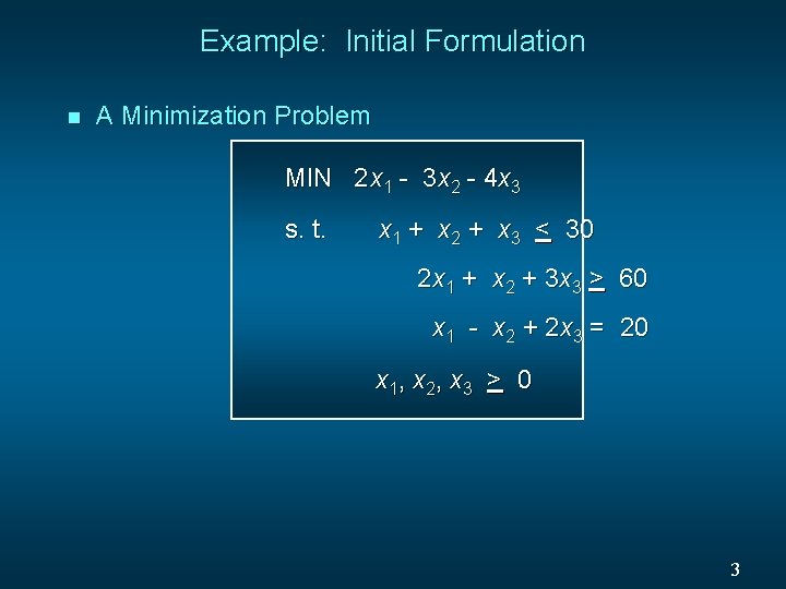
Example: Initial Formulation n A Minimization Problem MIN 2 x 1 - 3 x 2 - 4 x 3 s. t. x 1 + x 2 + x 3 < 30 2 x 1 + x 2 + 3 x 3 > 60 x 1 - x 2 + 2 x 3 = 20 x 1, x 2, x 3 > 0 3

Standard Form n n An LP is in standard form when: • All variables are non-negative • All constraints are equalities Putting an LP formulation into standard form involves: • Adding slack variables to “<“ constraints • Subtracting surplus variables from “>” constraints. 4

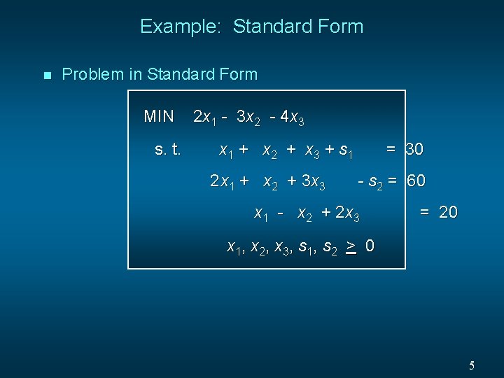
Example: Standard Form n Problem in Standard Form MIN s. t. 2 x 1 - 3 x 2 - 4 x 3 x 1 + x 2 + x 3 + s 1 2 x 1 + x 2 + 3 x 3 = 30 - s 2 = 60 x 1 - x 2 + 2 x 3 = 20 x 1, x 2, x 3, s 1, s 2 > 0 5

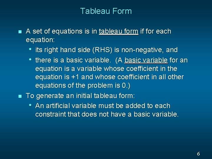
Tableau Form n n A set of equations is in tableau form if for each equation: • its right hand side (RHS) is non-negative, and • there is a basic variable. (A basic variable for an equation is a variable whose coefficient in the equation is +1 and whose coefficient in all other equations of the problem is 0. ) To generate an initial tableau form: • An artificial variable must be added to each constraint that does not have a basic variable. 6

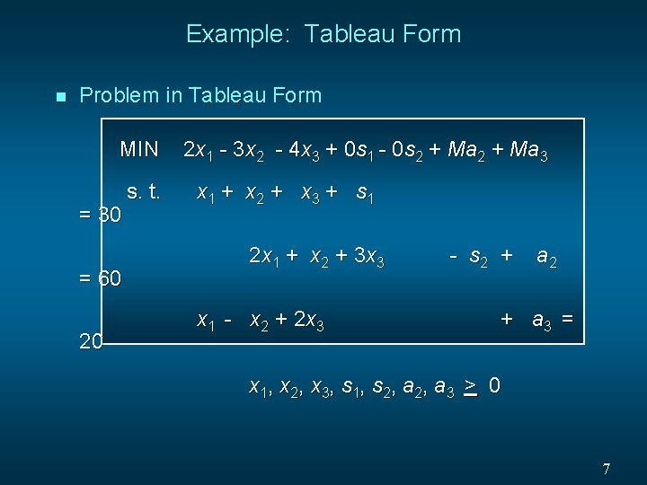
Example: Tableau Form n Problem in Tableau Form MIN = 30 = 60 20 s. t. 2 x 1 - 3 x 2 - 4 x 3 + 0 s 1 - 0 s 2 + Ma 3 x 1 + x 2 + x 3 + s 1 2 x 1 + x 2 + 3 x 3 x 1 - x 2 + 2 x 3 - s 2 + a 3 = x 1, x 2, x 3, s 1, s 2, a 3 > 0 7

Simplex Tableau n The simplex tableau is a convenient means for performing the calculations required by the simplex method. 8

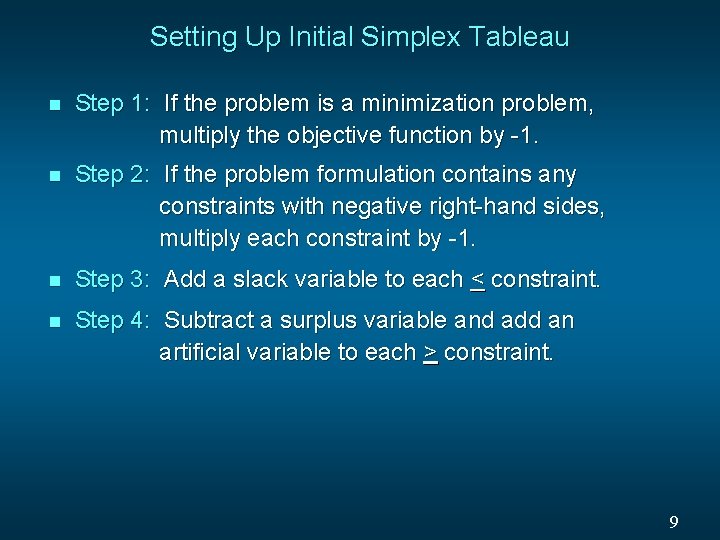
Setting Up Initial Simplex Tableau n Step 1: If the problem is a minimization problem, multiply the objective function by -1. n Step 2: If the problem formulation contains any constraints with negative right-hand sides, multiply each constraint by -1. n Step 3: Add a slack variable to each < constraint. n Step 4: Subtract a surplus variable and add an artificial variable to each > constraint. 9

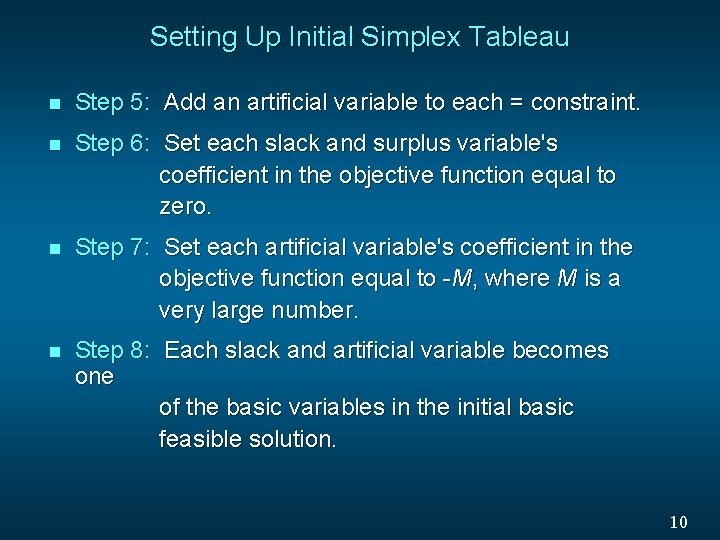
Setting Up Initial Simplex Tableau n Step 5: Add an artificial variable to each = constraint. n Step 6: Set each slack and surplus variable's coefficient in the objective function equal to zero. n Step 7: Set each artificial variable's coefficient in the objective function equal to -M, where M is a very large number. n Step 8: Each slack and artificial variable becomes one of the basic variables in the initial basic feasible solution. 10

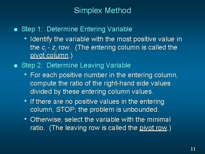
Simplex Method n n Step 1: Determine Entering Variable • Identify the variable with the most positive value in the cj - zj row. (The entering column is called the pivot column. ) Step 2: Determine Leaving Variable • For each positive number in the entering column, compute the ratio of the right-hand side values divided by these entering column values. • If there are no positive values in the entering column, STOP; the problem is unbounded. • Otherwise, select the variable with the minimal ratio. (The leaving row is called the pivot row. ) 11

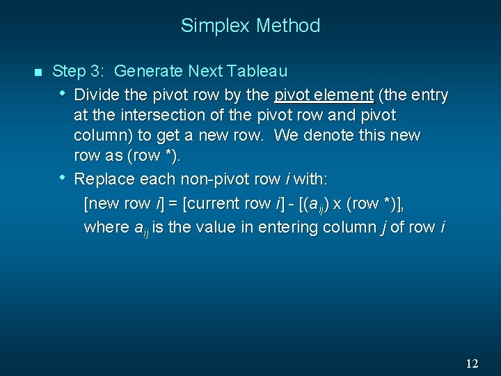
Simplex Method n Step 3: Generate Next Tableau • Divide the pivot row by the pivot element (the entry at the intersection of the pivot row and pivot column) to get a new row. We denote this new row as (row *). • Replace each non-pivot row i with: [new row i] = [current row i] - [(aij) x (row *)], where aij is the value in entering column j of row i 12

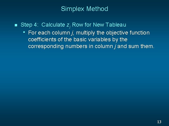
Simplex Method n Step 4: Calculate zj Row for New Tableau • For each column j, multiply the objective function coefficients of the basic variables by the corresponding numbers in column j and sum them. 13

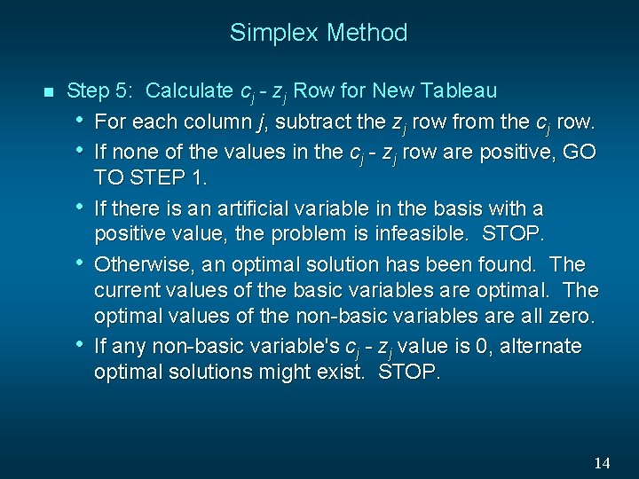
Simplex Method n Step 5: Calculate cj - zj Row for New Tableau • For each column j, subtract the zj row from the cj row. • If none of the values in the cj - zj row are positive, GO TO STEP 1. • If there is an artificial variable in the basis with a positive value, the problem is infeasible. STOP. • Otherwise, an optimal solution has been found. The current values of the basic variables are optimal. The optimal values of the non-basic variables are all zero. • If any non-basic variable's cj - zj value is 0, alternate optimal solutions might exist. STOP. 14

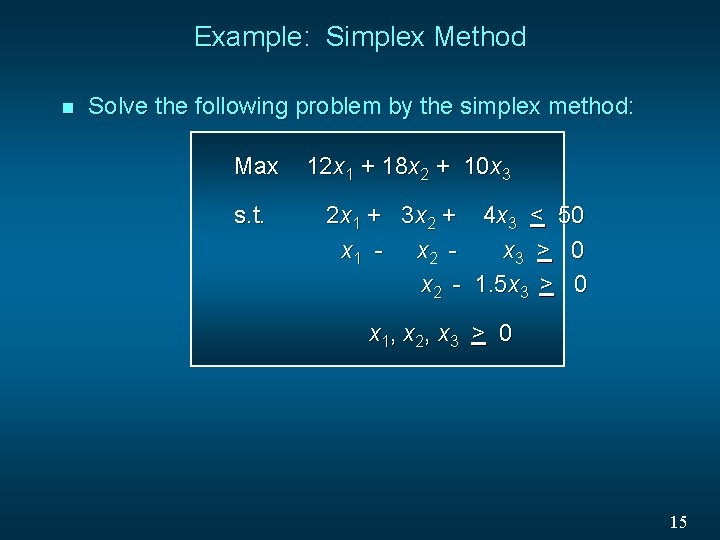
Example: Simplex Method n Solve the following problem by the simplex method: Max s. t. 12 x 1 + 18 x 2 + 10 x 3 2 x 1 + 3 x 2 + 4 x 3 < 50 x 1 - x 2 x 3 > 0 x 2 - 1. 5 x 3 > 0 x 1, x 2, x 3 > 0 15

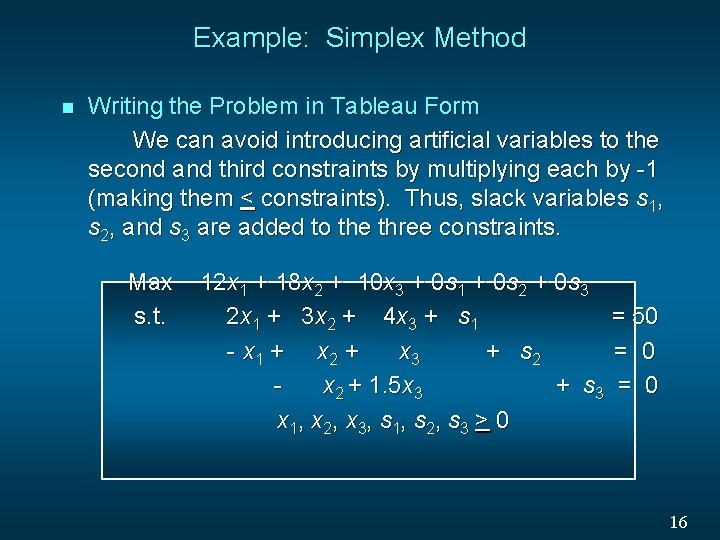
Example: Simplex Method n Writing the Problem in Tableau Form We can avoid introducing artificial variables to the second and third constraints by multiplying each by -1 (making them < constraints). Thus, slack variables s 1, s 2, and s 3 are added to the three constraints. Max s. t. 12 x 1 + 18 x 2 + 10 x 3 + 0 s 1 + 0 s 2 + 0 s 3 2 x 1 + 3 x 2 + 4 x 3 + s 1 = 50 - x 1 + x 2 + x 3 + s 2 = 0 x 2 + 1. 5 x 3 + s 3 = 0 x 1, x 2, x 3, s 1, s 2, s 3 > 0 16

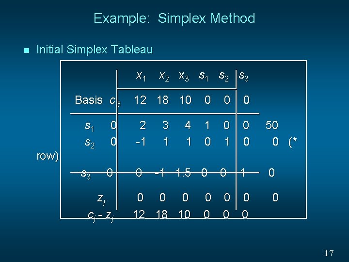
Example: Simplex Method n Initial Simplex Tableau x 1 Basis c. B row) s 1 s 2 s 3 0 0 0 zj cj - zj x 2 x 3 s 1 s 2 s 3 12 18 10 0 2 -1 1 0 0 50 0 (* 0 1 0 0 3 1 4 1 -1 1. 5 0 0 12 18 10 0 0 0 17

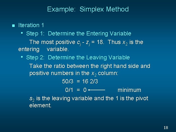
Example: Simplex Method n Iteration 1 • Step 1: Determine the Entering Variable The most positive cj - zj = 18. Thus x 2 is the entering variable. • Step 2: Determine the Leaving Variable Take the ratio between the right hand side and positive numbers in the x 2 column: 50/3 = 16 2/3 0/1 = 0 minimum s 2 is the leaving variable and the 1 is the pivot element. 18

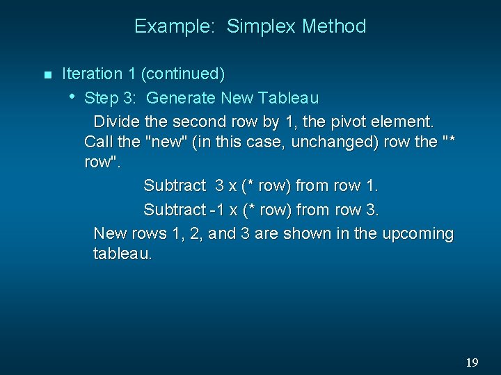
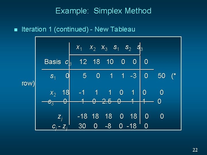
Example: Simplex Method n Iteration 1 (continued) • Step 3: Generate New Tableau Divide the second row by 1, the pivot element. Call the "new" (in this case, unchanged) row the "* row". Subtract 3 x (* row) from row 1. Subtract -1 x (* row) from row 3. New rows 1, 2, and 3 are shown in the upcoming tableau. 19

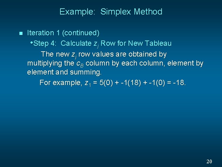
Example: Simplex Method n Iteration 1 (continued) • Step 4: Calculate zj Row for New Tableau The new zj row values are obtained by multiplying the c. B column by each column, element by element and summing. For example, z 1 = 5(0) + -1(18) + -1(0) = -18. 20

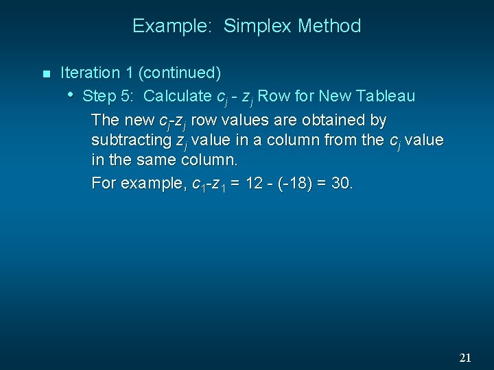
Example: Simplex Method n Iteration 1 (continued) • Step 5: Calculate cj - zj Row for New Tableau The new cj-zj row values are obtained by subtracting zj value in a column from the cj value in the same column. For example, c 1 -z 1 = 12 - (-18) = 30. 21

Example: Simplex Method n Iteration 1 (continued) - New Tableau x 1 Basis c. B row) s 1 x 2 x 3 s 1 s 2 s 3 12 18 10 0 5 x 2 18 s 3 0 -1 -1 zj cj - zj 0 1 0 0 0 1 -3 0 1 1 0 0 2. 5 0 1 1 0 1 -18 18 18 0 30 0 -8 0 -18 0 50 (* 0 0 0 22

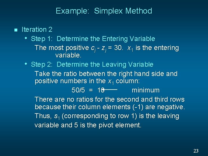
Example: Simplex Method n Iteration 2 • Step 1: Determine the Entering Variable The most positive cj - zj = 30. x 1 is the entering variable. • Step 2: Determine the Leaving Variable Take the ratio between the right hand side and positive numbers in the x 1 column: 50/5 = 10 minimum There are no ratios for the second and third rows because their column elements (-1) are negative. Thus, s 1 (corresponding to row 1) is the leaving variable and 5 is the pivot element. 23

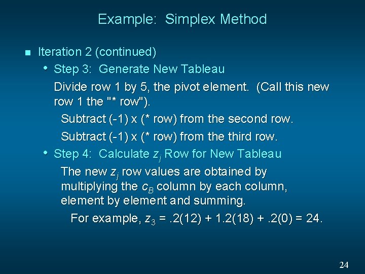
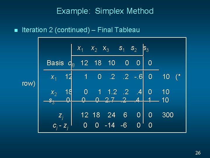
Example: Simplex Method n Iteration 2 (continued) • Step 3: Generate New Tableau Divide row 1 by 5, the pivot element. (Call this new row 1 the "* row"). Subtract (-1) x (* row) from the second row. Subtract (-1) x (* row) from the third row. • Step 4: Calculate zj Row for New Tableau The new zj row values are obtained by multiplying the c. B column by each column, element by element and summing. For example, z 3 =. 2(12) + 1. 2(18) +. 2(0) = 24. 24

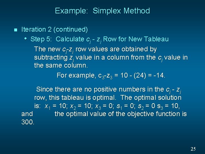
Example: Simplex Method n Iteration 2 (continued) • Step 5: Calculate cj - zj Row for New Tableau The new cj-zj row values are obtained by subtracting zj value in a column from the cj value in the same column. For example, c 3 -z 3 = 10 - (24) = -14. Since there are no positive numbers in the cj - zj row, this tableau is optimal. The optimal solution is: x 1 = 10; x 2 = 10; x 3 = 0; s 1 = 0; s 2 = 0 s 3 = 10, and the optimal value of the objective function is 300. 25

Example: Simplex Method n Iteration 2 (continued) – Final Tableau x 1 x 2 x 3 s 1 s 2 s 3 Basis c. B 12 18 10 row) x 1 12 1 x 2 s 3 18 0 0 0 zj cj - zj 0 . 2 0 0 0 . 2 -. 6 0 1 1. 2. 2. 4 0 0 2. 7. 2. 4 1 12 18 24 6 0 0 -14 -6 0 0 10 (* 10 10 300 26

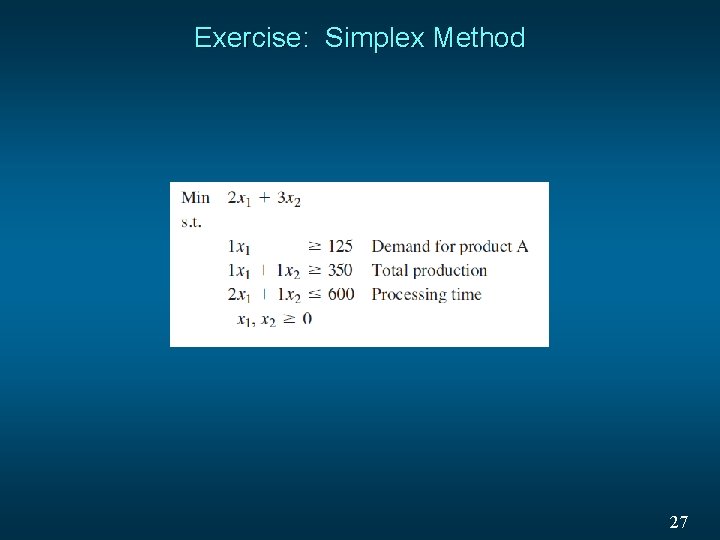
Exercise: Simplex Method 27

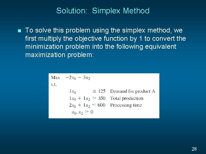
Solution: Simplex Method n To solve this problem using the simplex method, we first multiply the objective function by 1 to convert the minimization problem into the following equivalent maximization problem: 28

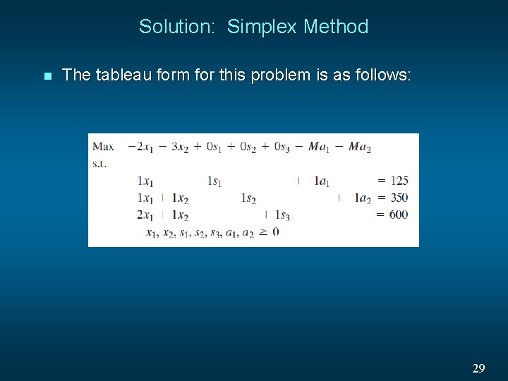
Solution: Simplex Method n The tableau form for this problem is as follows: 29

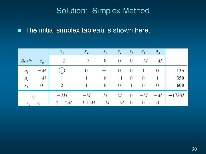
Solution: Simplex Method n The initial simplex tableau is shown here: 30

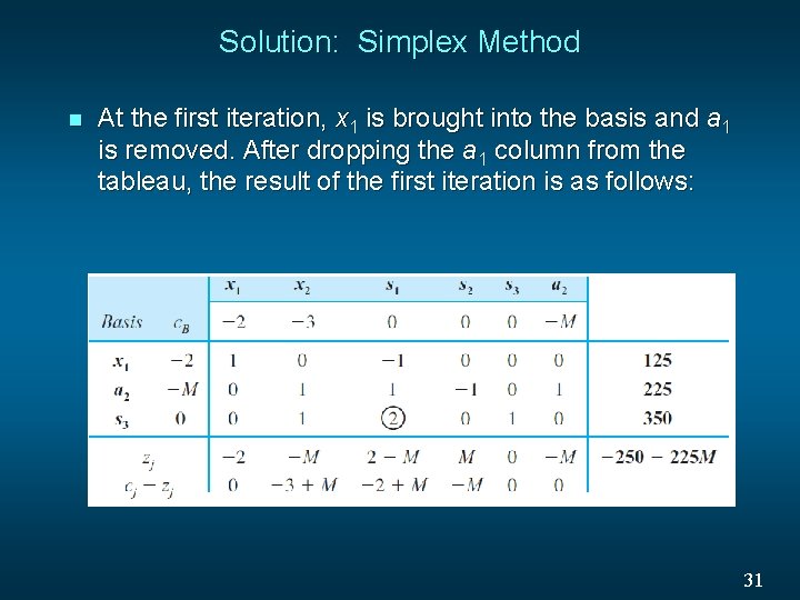
Solution: Simplex Method n At the first iteration, x 1 is brought into the basis and a 1 is removed. After dropping the a 1 column from the tableau, the result of the first iteration is as follows: 31

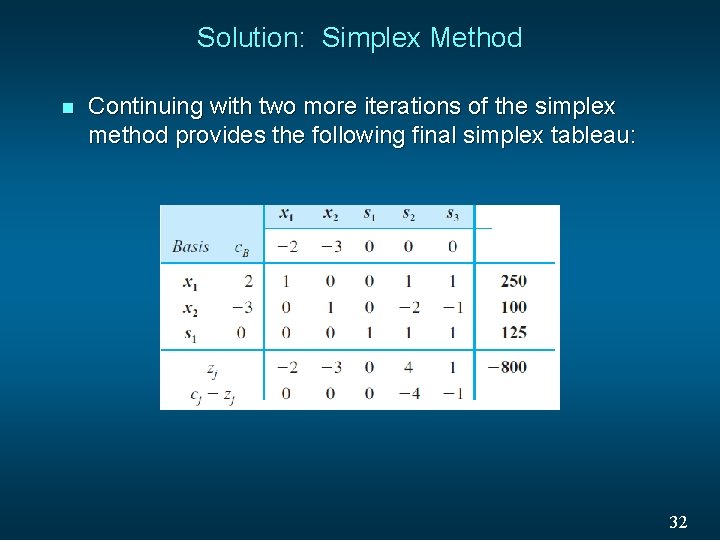
Solution: Simplex Method n Continuing with two more iterations of the simplex method provides the following final simplex tableau: 32

Special Cases n n Infeasibility Unboundedness Alternative Optimal Solution Degeneracy 33

Infeasibility n Infeasibility is detected in the simplex method when an artificial variable remains positive in the final tableau. 34

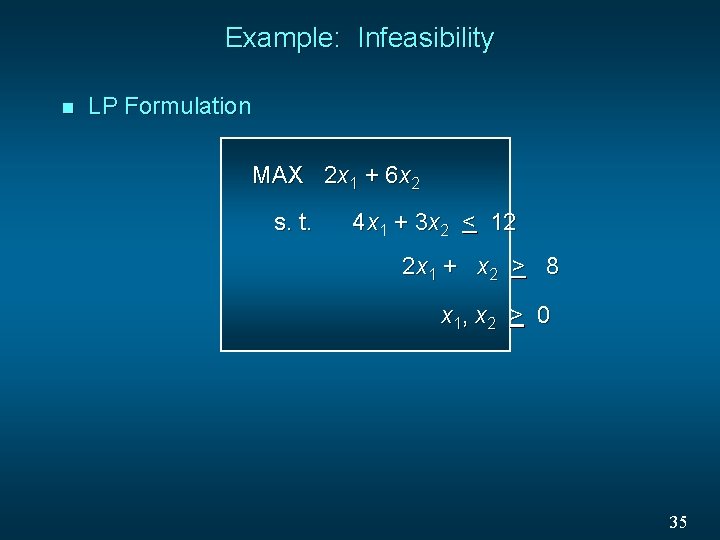
Example: Infeasibility n LP Formulation MAX 2 x 1 + 6 x 2 s. t. 4 x 1 + 3 x 2 < 12 2 x 1 + x 2 > 8 x 1, x 2 > 0 35

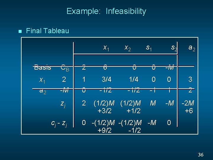
Example: Infeasibility n Final Tableau x 1 x 2 s 1 s 2 Basis CB 2 6 0 0 -M x 1 a 2 2 -M 1 0 3/4 -1/2 1/4 -1/2 0 -1 0 1 zj 2 (1/2)M +3/2 +1/2 M -M cj - zj 0 -(1/2)M -M +9/2 -1/2 a 2 3 2 -2 M +6 0 36

Example: Infeasibility In the previous slide we see that the tableau is the final tableau because all cj - zj < 0. However, an artificial variable is still positive, so the problem is infeasible. 37

Unboundedness n A linear program has an unbounded solution if all entries in an entering column are non-positive. 38

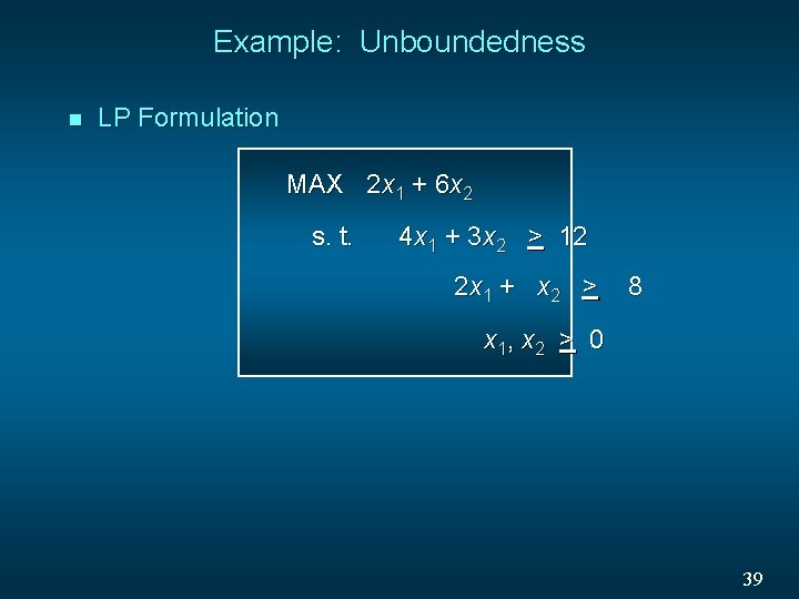
Example: Unboundedness n LP Formulation MAX 2 x 1 + 6 x 2 s. t. 4 x 1 + 3 x 2 > 12 2 x 1 + x 2 > 8 x 1, x 2 > 0 39

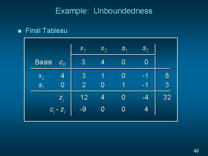
Example: Unboundedness n Final Tableau x 1 x 2 s 1 s 2 c. B 3 4 0 0 4 0 3 2 1 0 0 1 -1 -1 8 3 zj 12 4 0 -4 32 cj - zj -9 0 0 4 Basis x 2 s 1 40

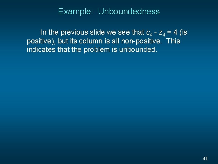
Example: Unboundedness In the previous slide we see that c 4 - z 4 = 4 (is positive), but its column is all non-positive. This indicates that the problem is unbounded. 41

Alternative Optimal Solution n A linear program has alternate optimal solutions if the final tableau has a cj - zj value equal to 0 for a nonbasic variable. 42

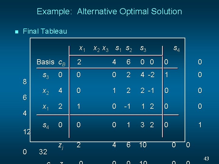
Example: Alternative Optimal Solution n Final Tableau x 1 Basis c. B 8 6 4 12 0 x 2 x 3 s 1 s 2 s 3 s 4 2 4 6 0 0 s 3 0 0 0 2 4 -2 1 0 x 2 4 0 1 2 2 -1 0 0 x 1 2 1 0 -1 1 2 0 0 s 4 0 0 0 1 3 2 0 1 zj 2 4 6 10 32 0 0 43

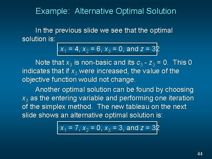
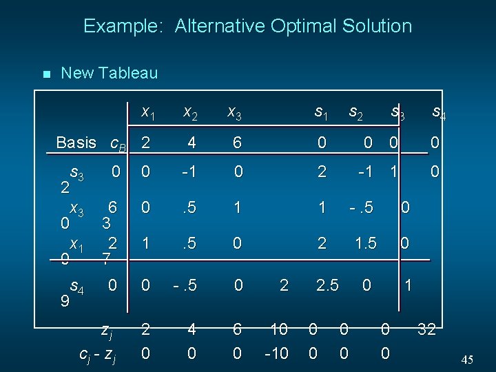
Example: Alternative Optimal Solution In the previous slide we see that the optimal solution is: x 1 = 4, x 2 = 6, x 3 = 0, and z = 32 Note that x 3 is non-basic and its c 3 - z 3 = 0. This 0 indicates that if x 3 were increased, the value of the objective function would not change. Another optimal solution can be found by choosing x 3 as the entering variable and performing one iteration of the simplex method. The new tableau on the next slide shows an alternative optimal solution is: x 1 = 7, x 2 = 0, x 3 = 3, and z = 32 44

Example: Alternative Optimal Solution n New Tableau x 1 x 2 x 3 s 1 s 2 s 3 Basis c. B 2 4 6 0 0 s 3 2 x 3 0 x 1 0 -1 1 0 0 0 -1 0 2 6 3 2 7 0 . 5 1 1 -. 5 0 1 . 5 0 2 1. 5 0 0 0 -. 5 0 2 0 1 zj cj - zj 2 0 4 0 6 0 10 -10 s 4 9 2. 5 0 0 0 s 4 32 45

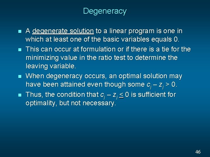
Degeneracy n n A degenerate solution to a linear program is one in which at least one of the basic variables equals 0. This can occur at formulation or if there is a tie for the minimizing value in the ratio test to determine the leaving variable. When degeneracy occurs, an optimal solution may have been attained even though some cj – zj > 0. Thus, the condition that cj – zj < 0 is sufficient for optimality, but not necessary. 46