CHAPTER 4 Laplace Transform EKT 232 1 Laplace

CHAPTER 4 Laplace Transform. EKT 232 1

Laplace Transform. 4. 1 4. 2 4. 3 4. 4 4. 5 Introduction. The Laplace Transform. The Unilateral Transform and Properties. Inversion of the Unilateral. Solving Differential Equation with Initial Conditions. 4. 6 Properties of the Bilateral Laplace Transform 4. 7 Properties of the Region of Convergence. 4. 8 Inversion of the Bilateral Laplace Transform. 4. 9 The Transfer Function 4. 10 Causality and Stability 2

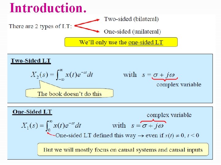
Introduction. þ In Chapter 3 we developed representation of signal and LTI by using superposition of complex sinusoids. þ In this Chapter 4 we are considering the continuous-time signal and system representation based on complex exponential signals. þ The Laplace transform can be used to analyze a large class of continuous-time problems involving signal that are not absolutely integrable, such as impulse response of an unstable system. þ Laplace transform come in two varieties; varieties (i) Unilateral (one sided); is a tool for solving differential equations with initial condition. (ii) Bilateral (two sided); offer insight into the nature of system characteristic such as stability, causality, and frequency response. 3

Introduction. 4

Pierre-Simon Laplace 3/23/1749 - 3/2/1827 6/15/2021 5

Laplace Transform Representation. þ H(s) is the Laplace Transform of h(t) and the h(t) is the inverse Laplace transform of H(s). þ The Laplace transform of x(t) is þ The Inverse Laplace Transform of X(s) is þ We can express the relationship with the notation 6

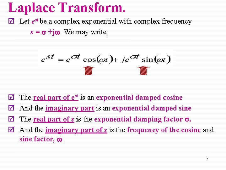
Laplace Transform. þ Let est be a complex exponential with complex frequency s = s +jw. We may write, þ þ The real part of est is an exponential damped cosine And the imaginary part is an exponential damped sine The real part of s is the exponential damping factor s. And the imaginary part of s is the frequency of the cosine and sine factor, w. 7

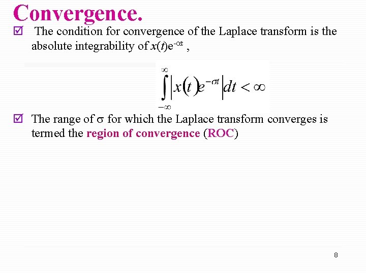
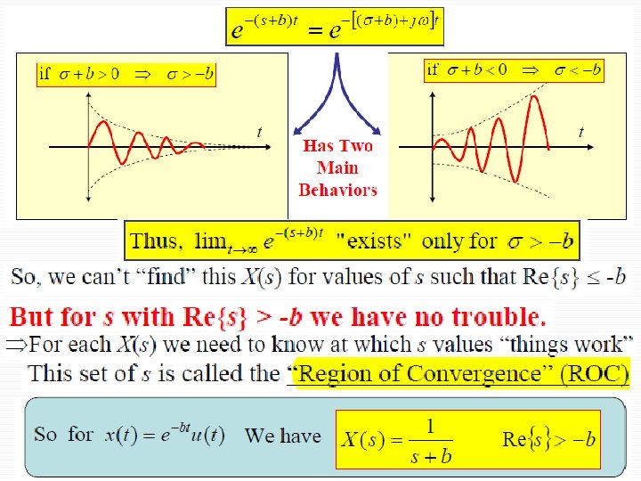
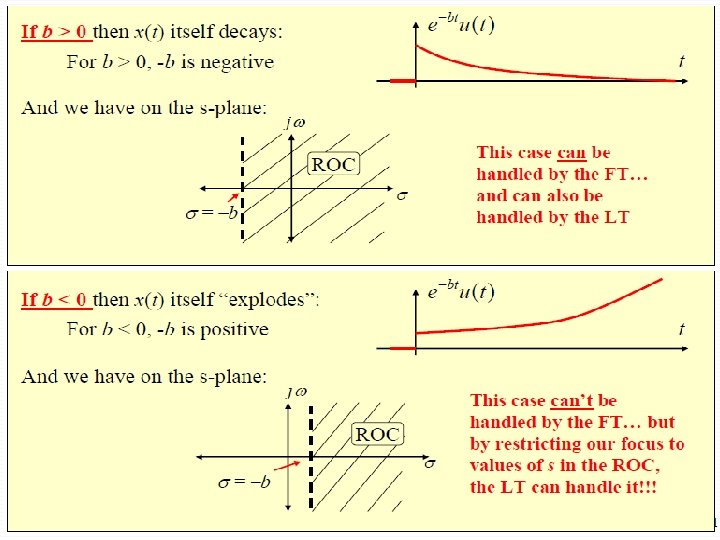
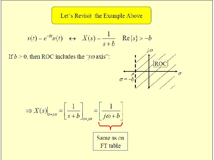
Convergence. þ The condition for convergence of the Laplace transform is the absolute integrability of x(t)e-at , þ The range of for which the Laplace transform converges is termed the region of convergence (ROC) 8

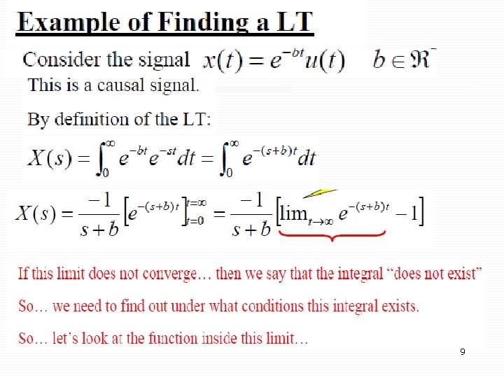
9

10

11

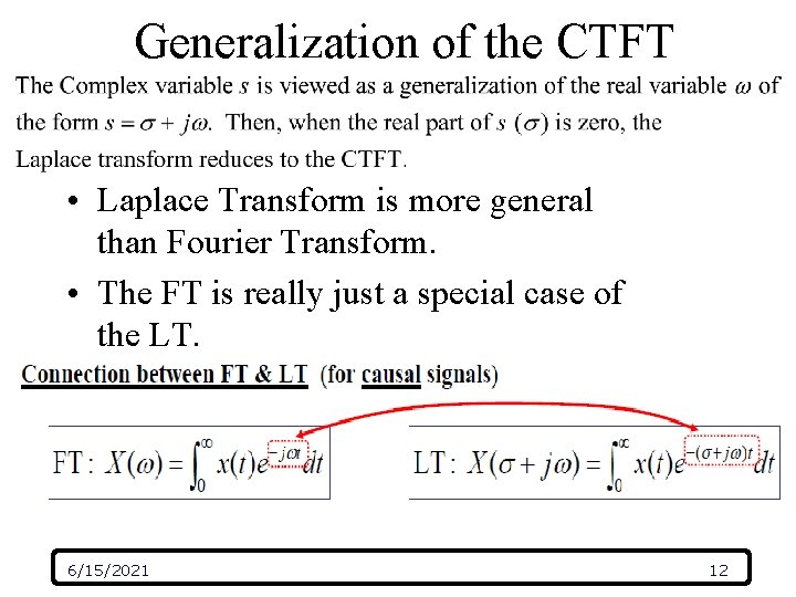
Generalization of the CTFT • Laplace Transform is more general than Fourier Transform. • The FT is really just a special case of the LT. 6/15/2021 12

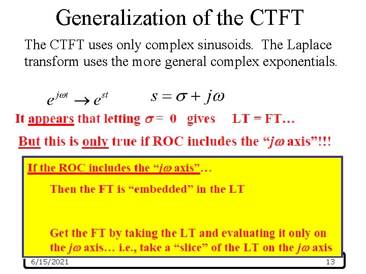
Generalization of the CTFT The CTFT uses only complex sinusoids. The Laplace transform uses the more general complex exponentials. 6/15/2021 13

Generalization of the CTFT 6/15/2021 14

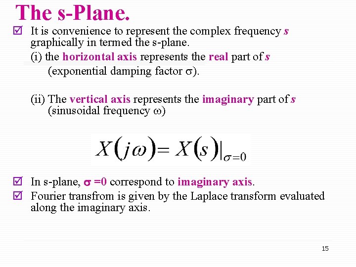
The s-Plane. þ It is convenience to represent the complex frequency s graphically in termed the s-plane. (i) the horizontal axis represents the real part of s (exponential damping factor ). (ii) The vertical axis represents the imaginary part of s (sinusoidal frequency w) þ In s-plane, s =0 correspond to imaginary axis. þ Fourier transfrom is given by the Laplace transform evaluated along the imaginary axis. 15

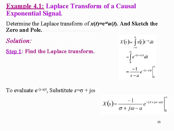
Example 4. 1: Laplace Transform of a Causal Exponential Signal. Determine the Laplace transform of x(t)=eatu(t). And Sketch the Zero and Pole. Solution: Step 1: Find the Laplace transform. To evaluate e-(s-a)t, Substitute s= + jw 16

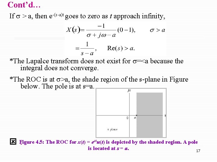
Cont’d… If > a, then e-(s-a)t goes to zero as t approach infinity, *The Lapalce transform does not exist for =<a because the integral does not converge. *The ROC is at >a, the shade region of the s-plane in Figure below. The pole is at s=a. 4. 5: The ROC for x(t) = eatu(t) is depicted by the shaded region. A pole ý Figure. is located at s = a. 17

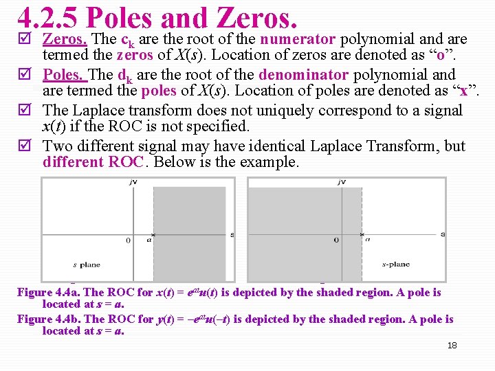
4. 2. 5 Poles and Zeros. þ Zeros. The ck are the root of the numerator polynomial and are termed the zeros of X(s). Location of zeros are denoted as “o”. þ Poles. The dk are the root of the denominator polynomial and are termed the poles of X(s). Location of poles are denoted as “x”. þ The Laplace transform does not uniquely correspond to a signal x(t) if the ROC is not specified. þ Two different signal may have identical Laplace Transform, but different ROC. Below is the example. Figure 6. 4 a Figure 6. 4 b Figure 4. 4 a. The ROC for x(t) = eatu(t) is depicted by the shaded region. A pole is located at s = a. Figure 4. 4 b. The ROC for y(t) = –eatu(–t) is depicted by the shaded region. A pole is located at s = a. 18

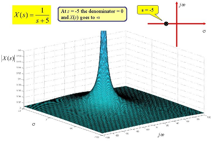
At s = -5 the denominator = 0 and X(s) goes to j s = -5 j

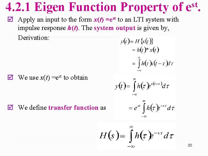
4. 2. 1 Eigen Function Property of est. þ Apply an input to the form x(t) =est to an LTI system with impulse response h(t). The system output is given by, Derivation: þ We use x(t) =est to obtain þ We define transfer function as 20

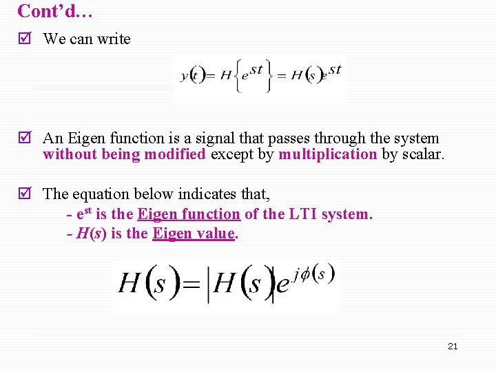
Cont’d… þ We can write þ An Eigen function is a signal that passes through the system without being modified except by multiplication by scalar. þ The equation below indicates that, - est is the Eigen function of the LTI system. - H(s) is the Eigen value. 21

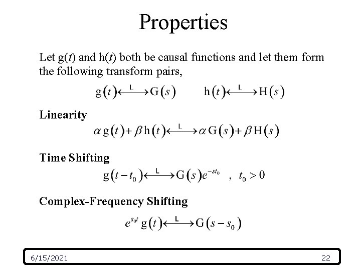
Properties Let g(t) and h(t) both be causal functions and let them form the following transform pairs, Linearity Time Shifting Complex-Frequency Shifting 6/15/2021 22

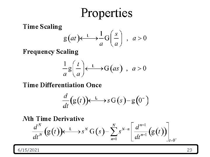
Properties Time Scaling Frequency Scaling Time Differentiation Once Nth Time Derivative 6/15/2021 23

Properties 6/15/2021 24

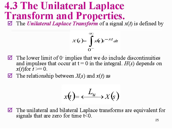
4. 3 The Unilateral Laplace Transform and Properties. þ The Unilateral Laplace Transform of a signal x(t) is defined by þ The lower limit of 0 - implies that we do include discontinuities and impulses that occur at t = 0 in the integral. H(s) depends on x(t)for t >= 0. þ The relationship between X(s) and x(t) as þ The unilateral and bilateral Laplace transforms are equivalent for signals that are zero for time t<0. 25

4. 4 Inversion of the Unilateral Laplace Transform. þ We can determine the inverse Laplace transforms using one-toone relationship between the signal and its unilateral Laplace transform. 26

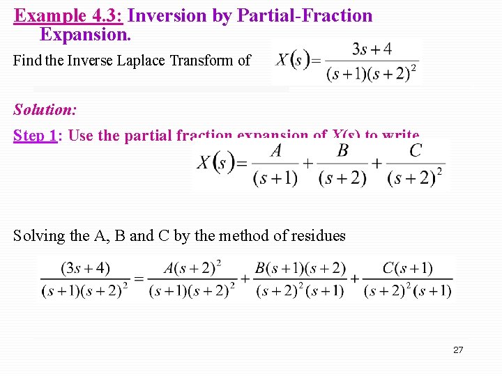
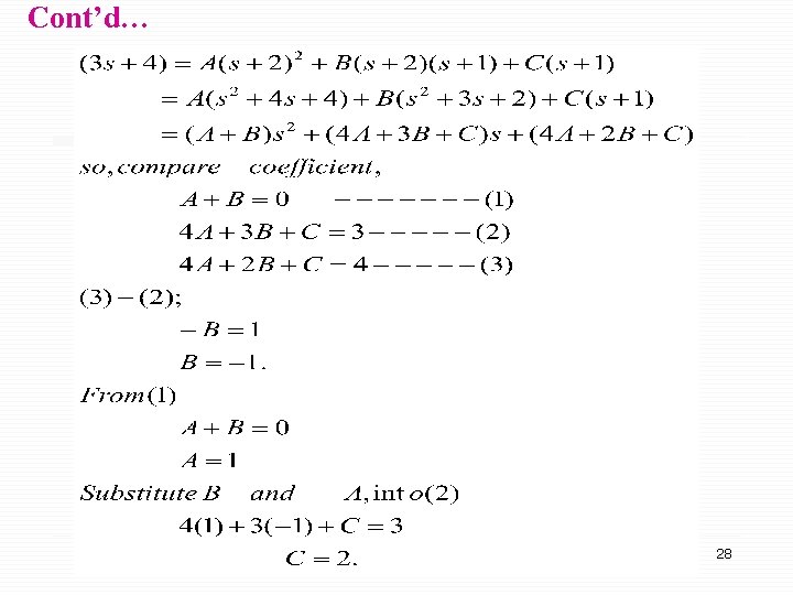
Example 4. 3: Inversion by Partial-Fraction Expansion. Find the Inverse Laplace Transform of Solution: Step 1: Use the partial fraction expansion of X(s) to write Solving the A, B and C by the method of residues 27

Cont’d… 28

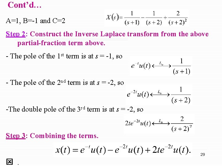
Cont’d… A=1, B=-1 and C=2 Step 2: Construct the Inverse Laplace transform from the above partial-fraction term above. - The pole of the 1 st term is at s = -1, so - The pole of the 2 nd term is at s = -2, so -The double pole of the 3 rd term is at s = -2, so Step 3: Combining the terms. 29 ý.

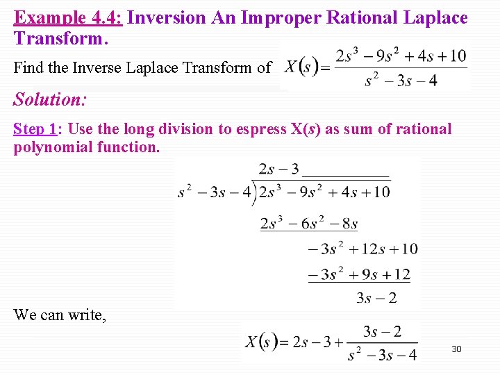
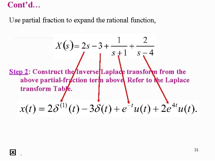
Example 4. 4: Inversion An Improper Rational Laplace Transform. Find the Inverse Laplace Transform of Solution: Step 1: Use the long division to espress X(s) as sum of rational polynomial function. We can write, 30

Cont’d… Use partial fraction to expand the rational function, Step 2: Construct the Inverse Laplace transform from the above partial-fraction term above. Refer to the Laplace transform Table. ý. 31

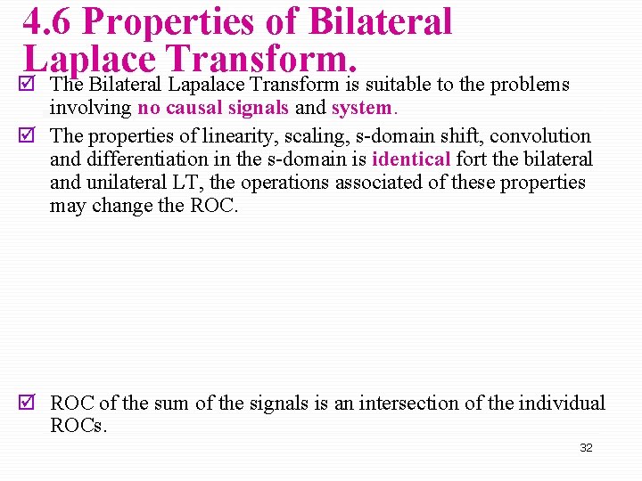
4. 6 Properties of Bilateral Laplace Transform. þ The Bilateral Lapalace Transform is suitable to the problems involving no causal signals and system. þ The properties of linearity, scaling, s-domain shift, convolution and differentiation in the s-domain is identical fort the bilateral and unilateral LT, the operations associated of these properties may change the ROC. þ ROC of the sum of the signals is an intersection of the individual ROCs. 32

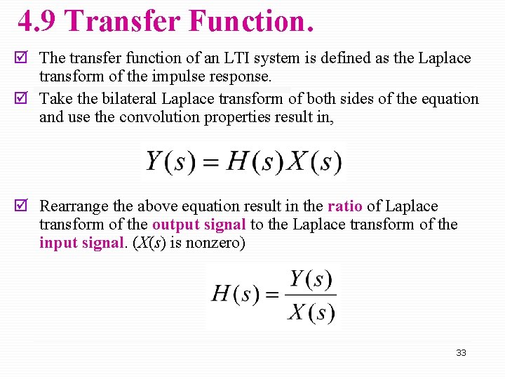
4. 9 Transfer Function. þ The transfer function of an LTI system is defined as the Laplace transform of the impulse response. þ Take the bilateral Laplace transform of both sides of the equation and use the convolution properties result in, þ Rearrange the above equation result in the ratio of Laplace transform of the output signal to the Laplace transform of the input signal. (X(s) is nonzero) 33

34

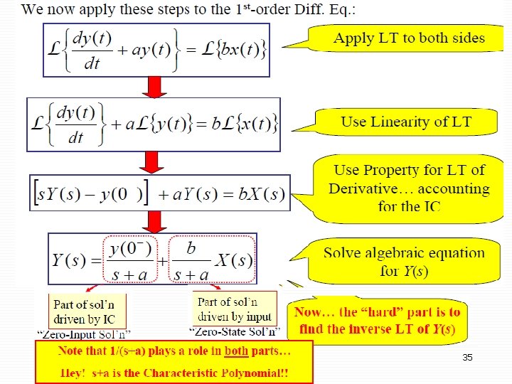
35

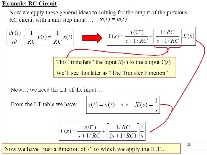
36

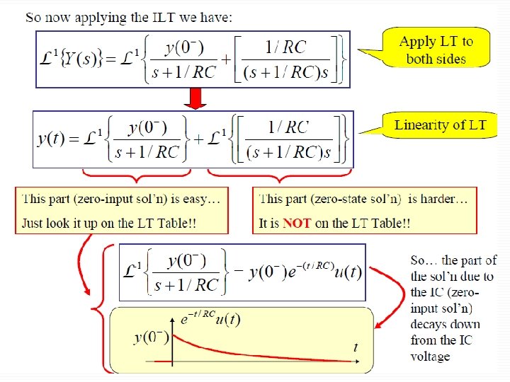
37

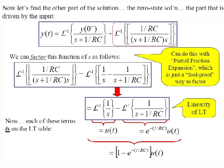
38

39

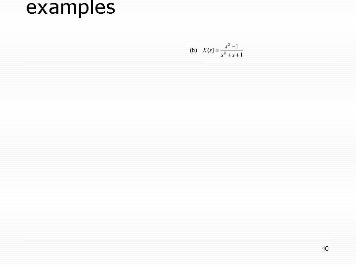
examples 40

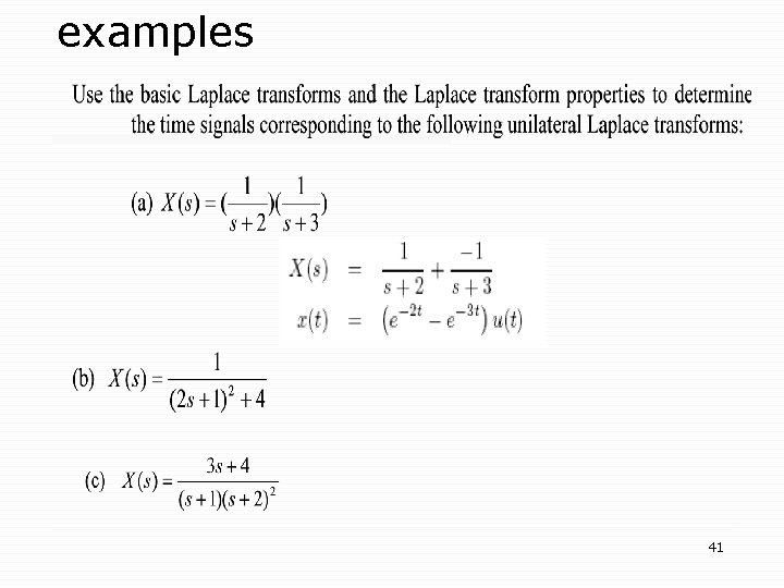
examples 41

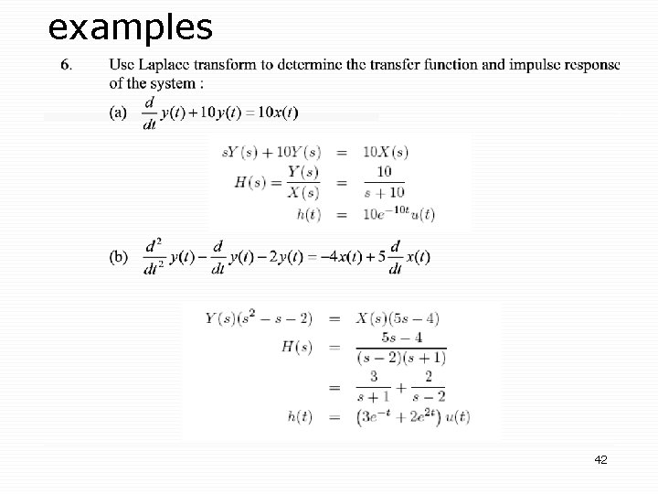
examples 42