Chapter 4 Informed Search Methods 4 1 4

Chapter 4 - Informed Search Methods 4. 1 4. 2 4. 3 4. 4 Best-First Search Heuristic Functions Memory Bounded Search Iterative Improvement Algorithms

4. 1 Best First Search Is just a General Search minimum-cost nodes are expanded first we basically choose the node that appears to be best according to the evaluation function Two basic approaches: Expand the node closest to the goal Expand the node on the least-cost solution path

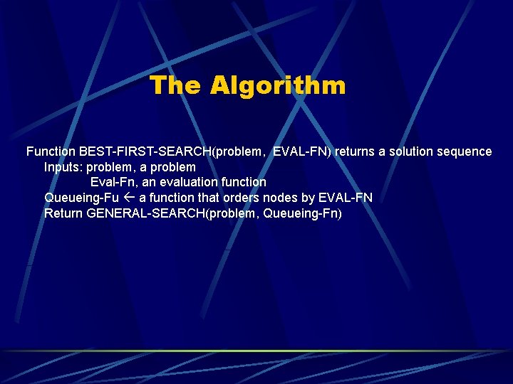
The Algorithm Function BEST-FIRST-SEARCH(problem, EVAL-FN) returns a solution sequence Inputs: problem, a problem Eval-Fn, an evaluation function Queueing-Fu a function that orders nodes by EVAL-FN Return GENERAL-SEARCH(problem, Queueing-Fn)

Greedy Search “ … minimize estimated cost to reach a goal” a heuristic function calculates such cost estimates h(n) = estimated cost of the cheapest path from the state at node n to a goal state

The Code Function GREEDY-SEARCH(problem) return a solution or failure return BEST-FIRST-SEARCH(problem, h) Required that h(n) = 0 if n = goal

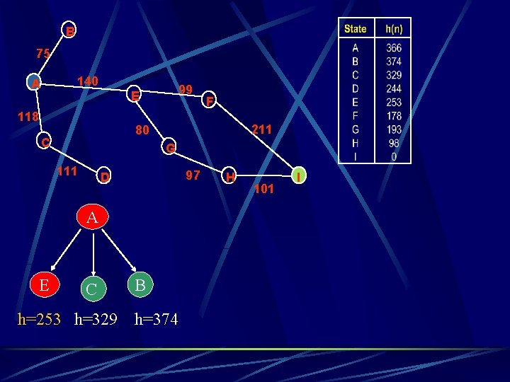
Straight-line distance The straight-line distance heuristic function is a for finding route-finding problem h. SLD(n) = straight-line distance between n and the goal location

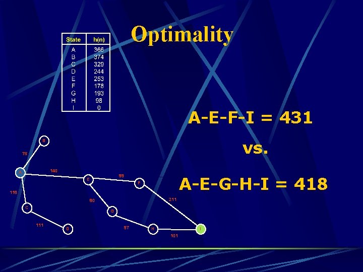
B 75 140 A 99 E 118 211 80 C G 111 97 D A E F C h=253 h=329 B h=374 H 101 I

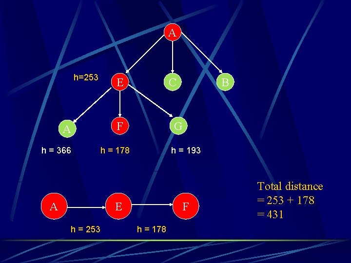
A h=253 A h = 366 A E C F G h = 178 h = 193 E h = 253 B F h = 178 Total distance = 253 + 178 = 431

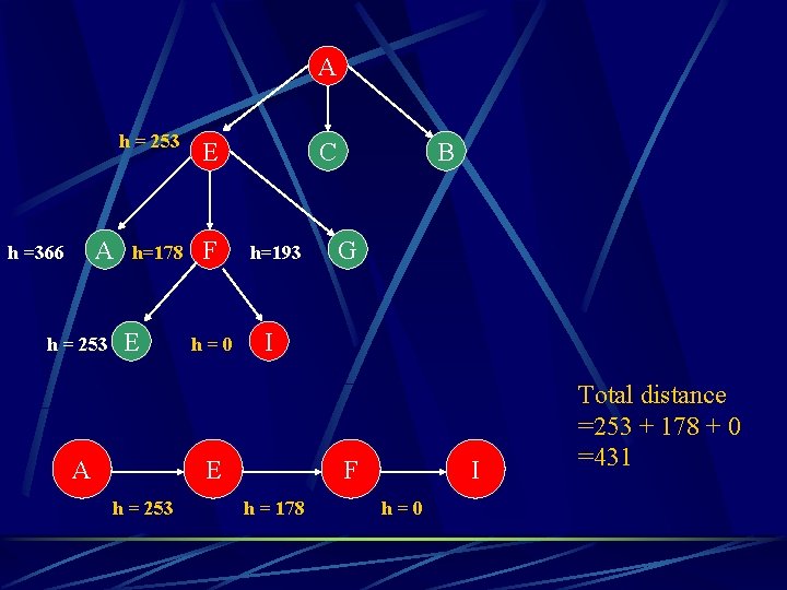
A A h =366 h = 253 E h=178 F E A h=0 C h=193 G I E h = 253 B F h = 178 I h=0 Total distance =253 + 178 + 0 =431

Optimality A-E-F-I = 431 vs. B 75 140 A 99 E A-E-G-H-I = 418 F 118 211 80 C G 111 D 97 H I 101

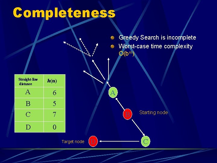
Completeness Greedy Search is incomplete Worst-case time complexity O(bm) Straight-line distance A h(n) B C 6 5 7 D 0 A B Target node D Starting node C

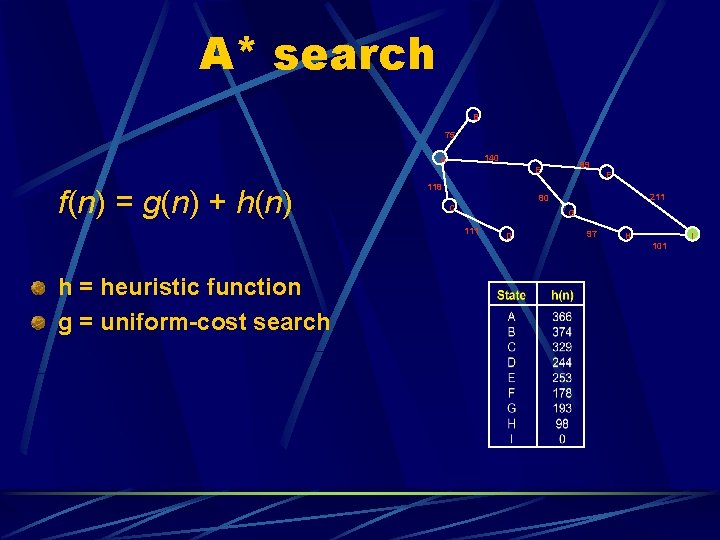
A* search B 75 140 A f(n) = g(n) + h(n) F 118 211 80 C G 111 h = heuristic function g = uniform-cost search 99 E D 97 H 101 I

“ Since g(n) gives the path from the start node to node n, and h(n) is the estimated cost of the cheapest path from n to the goal, we have… ” f(n) = estimated cost of the cheapest solution through n

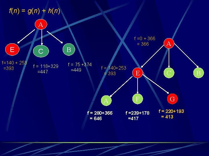
f(n) = g(n) + h(n) A E f=140 + 253 =393 C f = 118+329 =447 B f = 75 +374 =449 f = 140+253 = 393 A f = 280+366 = 646 f =0 + 366 = 366 A E C F G f =239+178 =417 f = 220+193 = 413 B

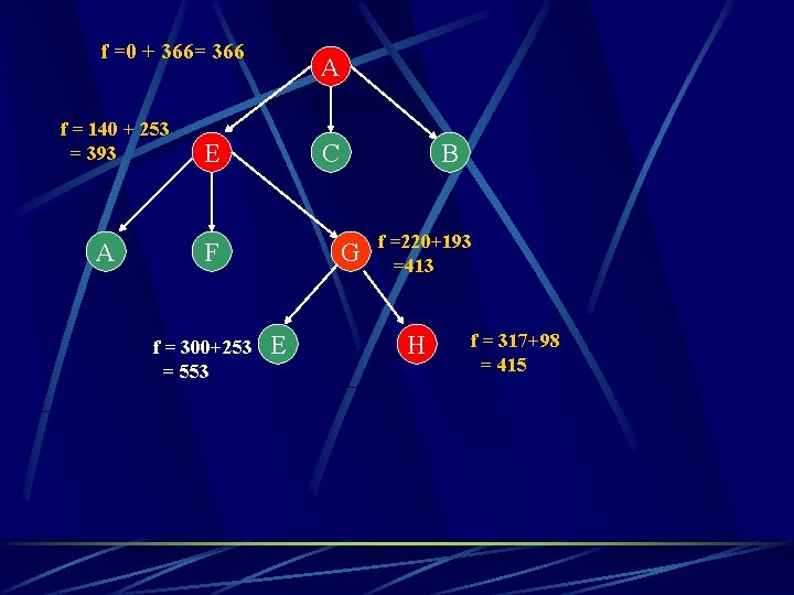
f =0 + 366= 366 f = 140 + 253 = 393 A A E C F f = 300+253 = 553 B G E f =220+193 =413 H f = 317+98 = 415

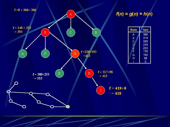
f =0 + 366= 366 f(n) = g(n) + h(n) A f = 140 + 253 = 393 E A F f = 300+253 = 553 C B G E f =220+193 =413 H f = 317+98 = 415 I f = 418+0 = 418

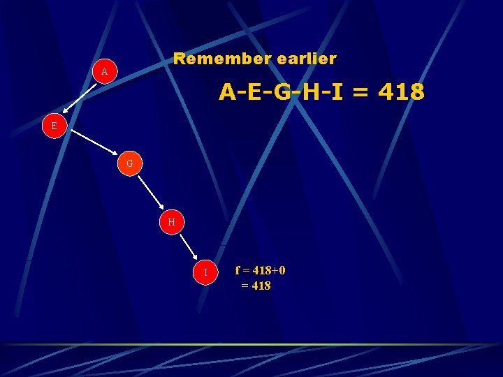
Remember earlier A A-E-G-H-I = 418 E G H I f = 418+0 = 418

The Algorithm function A*-SEARCH(problem) returns a solution or failure return BEST-FIRST-SEARCH(problem, g+h)

Chapter 4 - Informed Search Methods 4. 1 4. 2 4. 3 4. 4 Best-First Search Heuristic Functions Memory Bounded Search Iterative Improvement Algorithms

HEURISTIC FUNCTIONS

OBJECTIVE écalculates the cost estimates of an algorithm

IMPLEMENTATION é é é Greedy Search A* Search IDA*

EXAMPLES é é straight-line distance to B 8 -puzzle

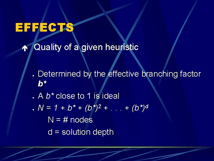
EFFECTS é Quality of a given heuristic l l l Determined by the effective branching factor b* A b* close to 1 is ideal N = 1 + b* + (b*)2 +. . . + (b*)d N = # nodes d = solution depth

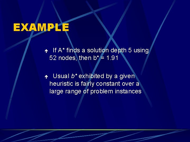
EXAMPLE é If A* finds a solution depth 5 using 52 nodes, then b* = 1. 91 é Usual b* exhibited by a given heuristic is fairly constant over a large range of problem instances

. . . A well-designed heuristic should have a b* close to 1. … allowing fairly large problems to be solved

NUMERICAL EXAMPLE Fig. 4. 8 Comparison of the search costs and effective branching factors for the IDA and A* algorithms with h 1, h 2. Data are averaged over 100 instances of the 8 -puzzle, for various solution lengths.

INVENTING HEURISTIC FUNCTIONS How ? • Depends on the restrictions of a given problem • A problem with lesser restrictions is known as a relaxed problem

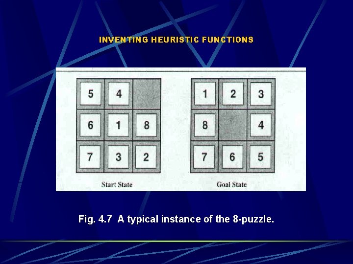
INVENTING HEURISTIC FUNCTIONS Fig. 4. 7 A typical instance of the 8 -puzzle.

INVENTING HEURISTIC FUNCTIONS One problem … one often fails to get one “clearly best” heuristic Given h 1, h 2, h 3, … , hm ; none dominates any others. Which one to choose ? h(n) = max(h 1(n), … , hm(n))

INVENTING HEURISTIC FUNCTIONS Another way: l l l performing experiment randomly on a particular problem gather results decide base on the collected information

HEURISTICS FOR CONSTRAINT SATISFACTION PROBLEMS (CSPs) most-constrained-variable least-constraining-value

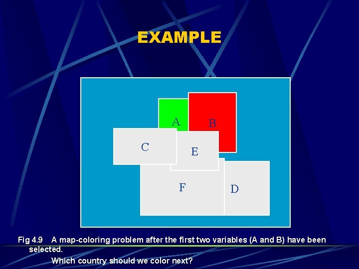
EXAMPLE A C B E F D Fig 4. 9 A map-coloring problem after the first two variables (A and B) have been selected. Which country should we color next?

Chapter 4 - Informed Search Methods 4. 1 4. 2 4. 3 4. 4 Best-First Search Heuristic Functions Memory Bounded Search Iterative Improvement Algorithms

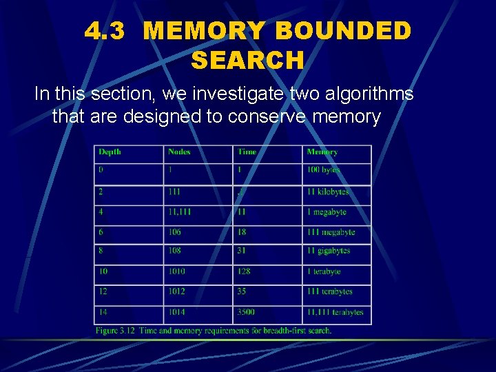
4. 3 MEMORY BOUNDED SEARCH In this section, we investigate two algorithms that are designed to conserve memory

Memory Bounded Search 1. IDA* (Iterative Deepening A*) search - is a logical extension of ITERATIVE - DEEPENING SEARCH to use heuristic information 2. SMA* (Simplified Memory Bounded A*) search

Iterative Deepening search Iterative Deepening is a kind of uniformed search strategy combines the benefits of depth- first and breadth-first search advantage - it is optimal and complete like breadth first search - modest memory requirement like depth-first search

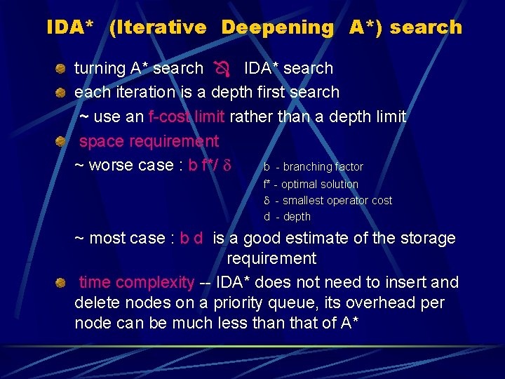
IDA* (Iterative Deepening A*) search turning A* search IDA* search each iteration is a depth first search ~ use an f-cost limit rather than a depth limit space requirement ~ worse case : b f*/ b - branching factor f* - optimal solution - smallest operator cost d - depth ~ most case : b d is a good estimate of the storage requirement time complexity -- IDA* does not need to insert and delete nodes on a priority queue, its overhead per node can be much less than that of A*

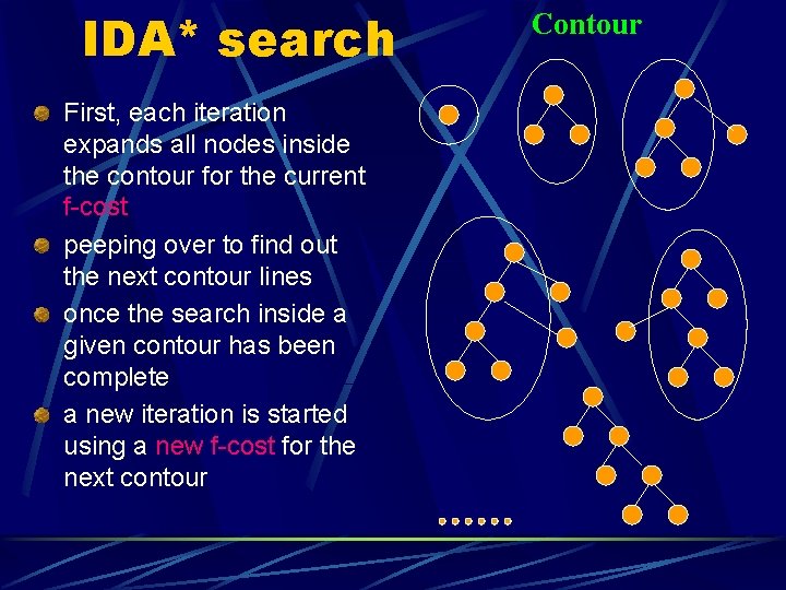
IDA* search First, each iteration expands all nodes inside the contour for the current f-cost peeping over to find out the next contour lines once the search inside a given contour has been complete a new iteration is started using a new f-cost for the next contour Contour

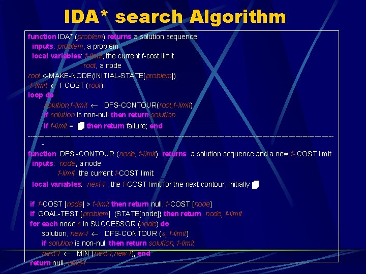
IDA* search Algorithm function IDA* (problem) returns a solution sequence inputs: problem, a problem local variables: f-limit, the current f-cost limit root, a node root <-MAKE-NODE(INITIAL-STATE[problem]) f-limit f-COST (root) loop do solution, f-limit DFS-CONTOUR(root, f-limit) if solution is non-null then return solution if f-limit = then return failure; end ----------------------------------------------------------------function DFS -CONTOUR (node, f-limit) returns a solution sequence and a new f- COST limit inputs: node, a node f-limit, the current f-COST limit local variables: next-f , the f-COST limit for the next contour, initially if f-COST [node] > f-limit then return null, f-COST [node] if GOAL-TEST [problem] (STATE[node]} then return node, f-limit for each node s in SUCCESSOR (node) do solution, new-f DFS-CONTOUR (s, f-limit) if solution is non-null then return solution, f-limit next-f MIN (next-f, new-f); end return null, next-f

MEMORY BOUNDED SEARCH 1. IDA* (Iterative Deepening A*) search 2. SMA* (Simplified Memory Bounded A*) search - is similar to A* , but restricts the queue size to fit into the available memory

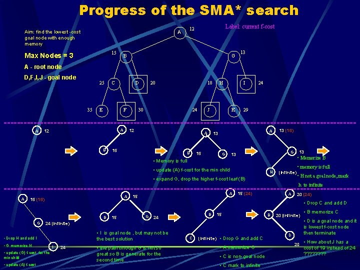
SMA* (Simplified Memory Bounded A*) Search advantage to use more memory -improve search efficiency Can make use of all available memory to carry out the search remember a node rather than to regenerate it when needed

SMA* search (cont. ) SMA* has the following properties SMA* will utilize whatever memory is made available to it SMA* avoids repeated states as far as its memory allows SMA* is complete if the available memory is sufficient to store the shallowest solution path

SMA* search (cont. ) SMA* properties cont. SMA* is optimal if enough memory is available to store the shallowest optimal solution path when enough memory is available for the entire search tree, the search is optimally efficient

Progress of the SMA* search Aim: find the lowest -cost goal node with enough memory 15 Max Nodes = 3 Label: current f-cost 12 A B G 13 A - root node D, F, I, J - goal node 25 35 C D E F 20 18 30 24 H I J K 24 29 -----------------------------------------------------A 12 B 15 B A 13 A 15 G 13 (15) 13 G 13 • Memorize B • Memory is full • update (A) f-cost for the min child • memory is full H (Infinite) • expand G, drop the higher f-cost leaf (B) • H not a goal node, mark h to infinite ------------------------------------------------------15 (24) 20 (24) A A 15 (15) • G memorize H • update (G) f-cost for the • update (A) f-cost 15 G B 24 15 B 20 (infinite) • I is goal node , but may not be the best solution I 24 • the path through G is not so great so B is generate for the second time C (Infinite) • Drop G and add C • A memorize G • C is non-goal node • C mark to infinite • B memorize C • D is a goal node and it is lowest f-cost node then terminate 24 (infinite) • Drop H and add I min child A • Drop C and add D B G A 15 D 20 • How about J has a cost of 19 instead of 24 ? ? ? ?

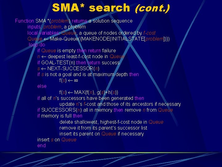
SMA* search (cont. ) Function SMA *(problem) returns a solution sequence inputs: problem, a problem local variables: Queue, a queue of nodes ordered by f-cost Queue Make-Queue({MAKENODE(INITIALSTATE[problem])}) loop do if Queue is empty then return failure n deepest least-f-cost node in Queue if GOAL-TEST(n) then return success s NEXT-SUCCESSOR(n) if s is not a goal and is at maximum depth then f(s) else f(s) MAX(f(n), g(s)+h(s)) if all of n’s successors have been generated then update n’s f-cost and those of its ancestors if necessary if SUCCESSORS(n) all in memory then remove n from Queue if memory is full then delete shallowest, highest-f-cost node in Queue remove it from its parent’s successor list insert its parent on Queue if necessary insert s on Queue end

Chapter 4 - Informed Search Methods 4. 1 4. 2 4. 3 4. 4 Best-First Search Heuristic Functions Memory Bounded Search Iterative Improvement Algorithms

ITERATIVE IMPROVEMENT ALGORITHMS For the most practical approach in which All the information needed for a solution are contained in the state description itself The path of reaching a solution is not important Advantage: memory save by keeping track of only the current state Two major classes: Hill-climbing (gradient descent) Simulated annealing

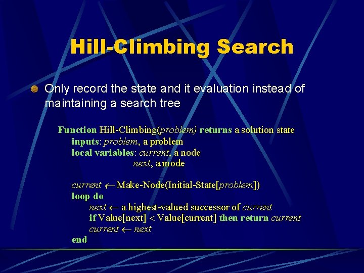
Hill-Climbing Search Only record the state and it evaluation instead of maintaining a search tree Function Hill-Climbing(problem) returns a solution state inputs: problem, a problem local variables: current, a node next, a mode current Make-Node(Initial-State[problem]) loop do next a highest-valued successor of current if Value[next] Value[current] then return current next end

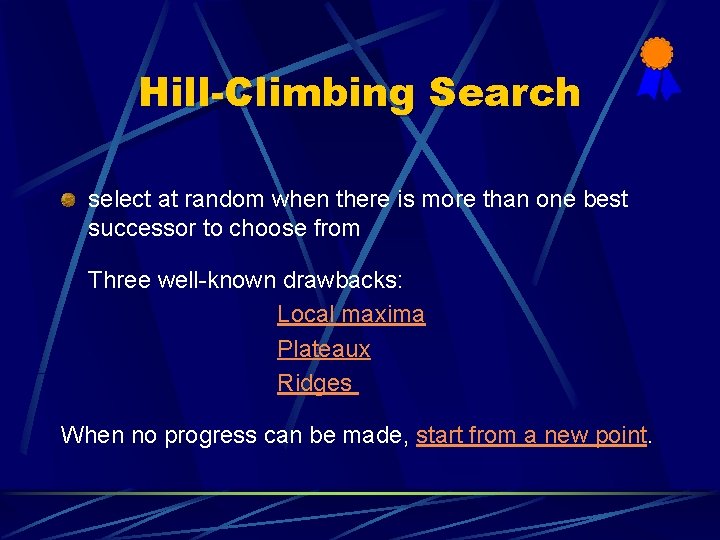
Hill-Climbing Search select at random when there is more than one best successor to choose from Three well-known drawbacks: Local maxima Plateaux Ridges When no progress can be made, start from a new point.

Local Maxima A peak lower than the highest peak in the state space The algorithm halts when a local maximum is reached

Plateaux Neighbors of the state are about the same height A random walk will be generated

Ridges No steep sloping sides between the top and peaks The search makes little progress unless the top is directly reached

Random-Restart Hill-Climbing Generates different starting points when no progress can be made from the previous point Saves the best result Can eventually find out the optimal solution if enough iterations are allowed The fewer local maxima, the quicker it finds a good solution

Simulated Annealing Picks random moves Keeps executing the move if the situation is actually improved; otherwise, makes the move of a probability less than 1 Number of cycles in the search is determined according to probability The search behaves like hill-climbing when approaching the end Originally used for the process of cooling a liquid

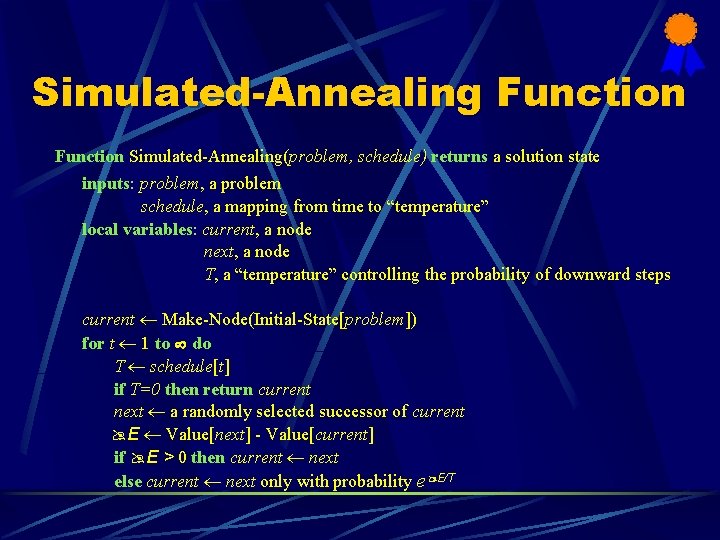
Simulated-Annealing Function Simulated-Annealing(problem, schedule) returns a solution state inputs: problem, a problem schedule, a mapping from time to “temperature” local variables: current, a node next, a node T, a “temperature” controlling the probability of downward steps current Make-Node(Initial-State[problem]) for t 1 to do T schedule[t] if T=0 then return current next a randomly selected successor of current E Value[next] - Value[current] if E > 0 then current next else current next only with probability e E/T

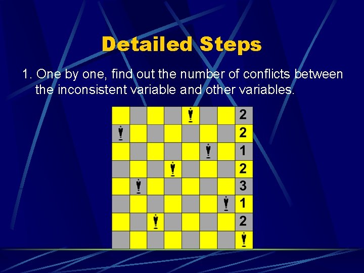
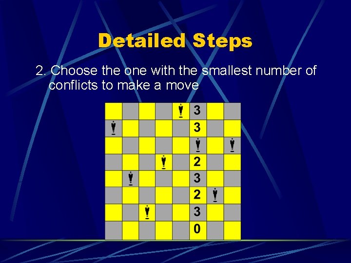
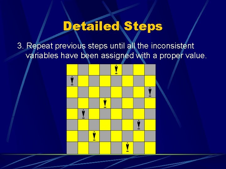
Applications in Constraint Satisfaction Problems General algorithms for Constraint Satisfaction Problems assigns values to all variables applies modifications to the current configuration by assigning different values to variables towards a solution Example problem: an 8 -queens problem (Definition of an 8 -queens problem is on Pg 64, text)

An 8 -queens Problem Algorithm chosen: the min-conflicts heuristic repair method Algorithm Characteristics: repairs inconsistencies in the current configuration selects a new value for a variable that results in the minimum number of conflicts with other variables

Detailed Steps 1. One by one, find out the number of conflicts between the inconsistent variable and other variables.

Detailed Steps 2. Choose the one with the smallest number of conflicts to make a move

Detailed Steps 3. Repeat previous steps until all the inconsistent variables have been assigned with a proper value.