Chapter 4 Human Resource Development Education 4 1
- Slides: 22

Chapter 4 Human Resource Development : Education 4. 1 Is education an investment good or consumption good? 4. 2 Is education a private or public goods ? 4. 3 Is education an individual demand or public demand? 4. 4 Assumption and Investment 4. 5 Saving (i) VS Education (r) 4. 6 Relation between education , age and earning

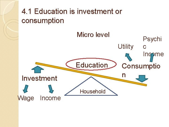
4. 1 Education is investment or consumption Micro level Utility Education Investment Wage Income Household Psychi c Income Consumptio n

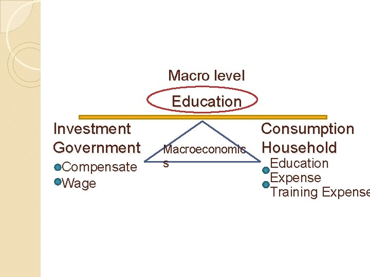
Macro level Education Investment Government Compensate Wage Macroeconomic s Consumption Household Education Expense Training Expense

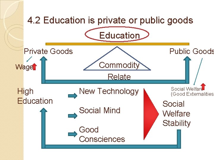
4. 2 Education is private or public goods Education Private Goods Wage High Education Public Goods Commodity Relate New Technology Social Mind Good Consciences Social Welfare (Good Externalities) Externalities Social Welfare Stability

Ex. 4. 1 Public Goods Assumption of Public Goods 1. Open access 2. One consume do not obstruct or decrease consume from others Ex. Case of “Satellite” If government setting the free satellite that everyone can access with free of charge. One household access to this system disturb others.

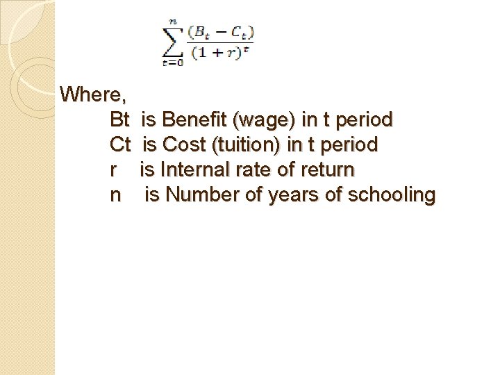
4. 3 Education is individual demand or public demand A) Individual demand of education Compare to commodity in the market, x, we have demand for x at Px and Qx Individual demand of education, we have demand for education x years of schooling and we have to pay for tuition fee. Later, we gain educational internal rate of return “r”

Where, Bt Ct r n is Benefit (wage) in t period is Cost (tuition) in t period is Internal rate of return is Number of years of schooling

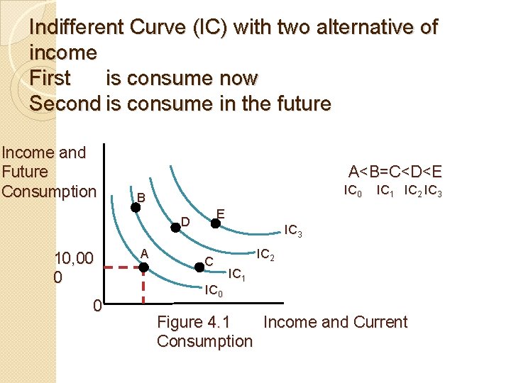
Indifferent Curve (IC) with two alternative of income First is consume now Second is consume in the future Income and Future Consumption A<B=C<D<E IC 0 B E D 10, 00 0 0 A IC 1 IC 2 IC 3 C IC 0 IC 2 IC 1 Figure 4. 1 Income and Current Consumption

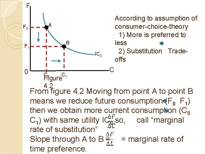
F F 0 According to assumption of consumer-choice-theory 1) More is preferred to less 2) Substitution Tradeoffs A B F 1 IC 0 0 C 1 Figure 4. 2 C From figure 4. 2 Moving from point A to point B means we reduce future consumption (F 0 F 1) then we obtain more current consumption (C 0 C 1) with same utility IC 0 so, call “marginal rate of substitution” Slope through A to B = = marginal rate of time preference.

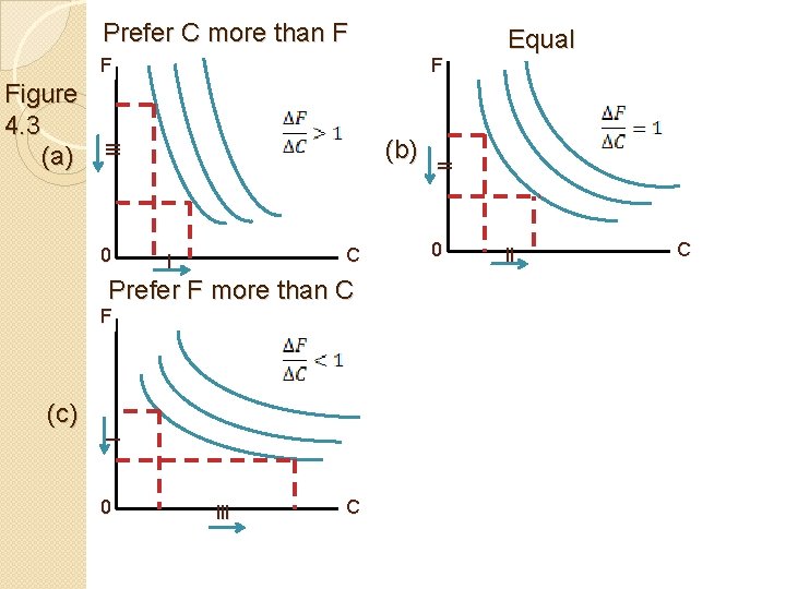
Prefer C more than F F 0 C l Prefer F more than C F (c) l 0 lll C ll (b) lll Figure 4. 3 (a) F Equal 0 ll C

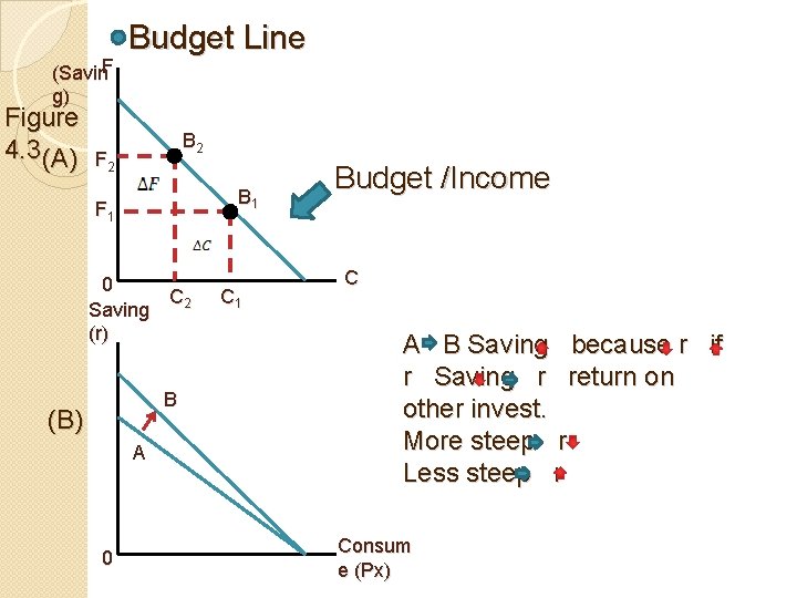
(Savin. F g) Figure 4. 3(A) Budget Line B 2 F 2 B 1 F 1 0 C 2 Saving (r) B (B) A 0 C 1 Budget /Income C A B Saving because r if r Saving r return on other invest. More steep r Less steep r Consum e (Px)

Figure 4. 3 shows the total income of individual i who can allocate his/her money to consume now or future. B 0 present no saving, almost consume now, B 1 show saving and consume at F 1 , C 1 respectively. If he/she at B 1 is present initial point, consume C 1 and saving F 1 when he reduce his consumption from C 1 to C 2 (∆C) then, He has transferred his money to saving with ∆F and obtain “I” interest rate. so, he obtain saving amount = ∆F(1+i) Conclude that B 0 No saving consume 100%

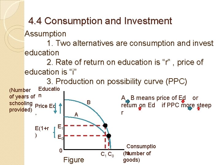
4. 4 Consumption and Investment Assumption 1. Two alternatives are consumption and invest education 2. Rate of return on education is “r” , price of education is “i” 3. Production on possibility curve (PPC) (Number Educatio of years of n schooling Price Ed provided) , E(1+r ) A B means price of Ed or return on Ed if PPC more steep r B A E 1 E 0 0 Figure C 1 C 0 Consumptio n (Number of goods)

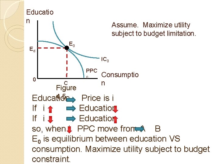
Educatio n Assume. Maximize utility subject to budget limitation. E 0 Ed IC 0 PPC 0 0 C Consumptio n Figure 4. 5 Education Price is i If i Education so, when i PPC move from A B E 0 is equilibrium between education VS consumption. Maximize utility subject to budget constraint.

4. 5 Saving (i) VS Education (r) Assumption 1. Saving and education are substitution goods 2. Opportunity cost of saving is return on education (r) 3. Opportunity cost of education is return on saving (i) 4. Price of saving is r 5. Price of education is i 6. Saving and education are normal goods

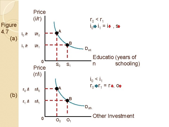
Figure 4. 7 (a) Price (i/r) i 0 /r i/r 0 i 1 /r i/r 1 A B Ded. 0 Price (r/i) (b) r 0 /i r/i 0 r 1 /i r/i 1 r 0 < r 1 i 0 i 1 = i , s S 0 Educatio (years of n schooling) S 1 i 0 < i 1 r 0 r 1 = r , o A B Doth. 0 O 1 Other Investment

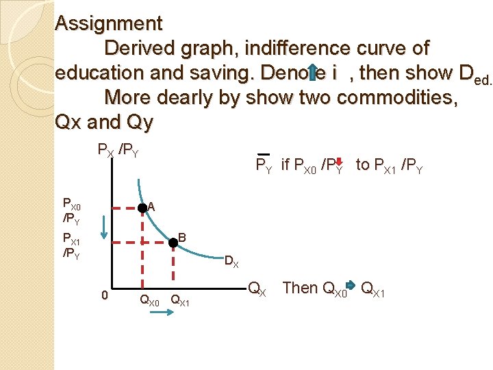
Assignment Derived graph, indifference curve of education and saving. Denote i , then show Ded. More dearly by show two commodities, Qx and Qy PX /PY PX 0 /PY PY if PX 0 /PY to PX 1 /PY A B PX 1 /PY DX 0 QX 1 QX Then QX 0 QX 1

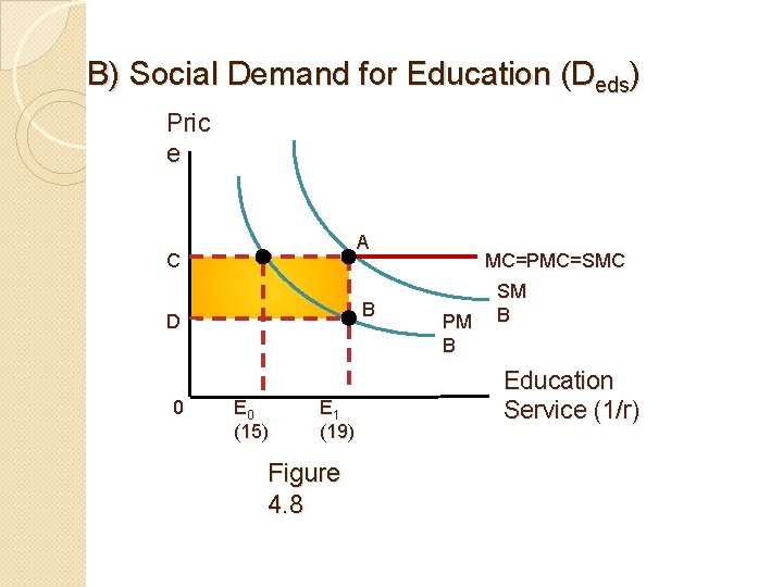
B) Social Demand for Education (Deds) Pric e A C B D 0 E 0 (15) E 1 (19) Figure 4. 8 MC=PMC=SMC PM B SM B Education Service (1/r)

Assumption 1. Marginal cost of education constant and equal to private MC, social MC. ˙. MC=PMC=SMC= constant. Education Positivemarginal to socialbenefit Figure 2. 4. 8 shows that private externalities (PMB) or individual demand for education is less than social expectation. For instance, E 0 is a 15 years of schooling while E 1 is 19 years (university). Parent seems to invest their kids only secondary school not university. But social benefit occur if population graduate at least university level (under graduation). Therefore, CABD should support by government or subsidy for tuition fee student loan, Scholarship.

Discussion • What level should supported by parent. • What level should supported by government. Assignment Find research paper related to this point and present for 5 minute.

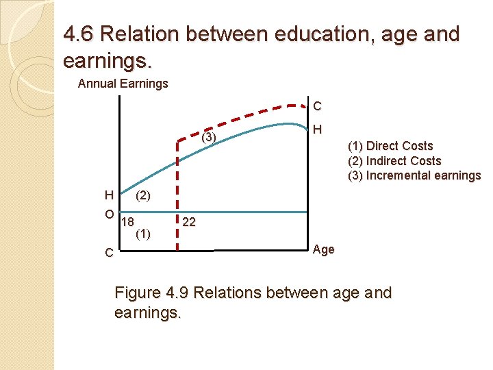
4. 6 Relation between education, age and earnings. Annual Earnings C (3) H O C H (1) Direct Costs (2) Indirect Costs (3) Incremental earnings (2) 18 (1) 22 Age Figure 4. 9 Relations between age and earnings.

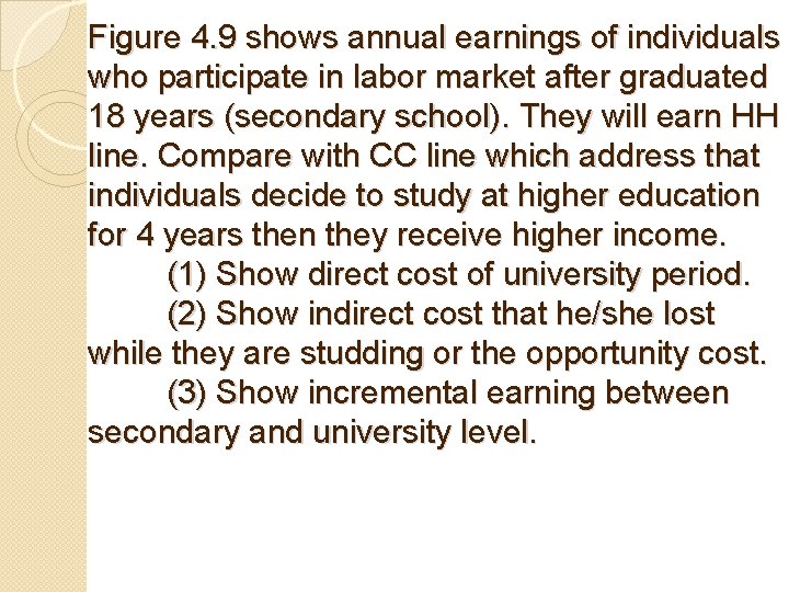
Figure 4. 9 shows annual earnings of individuals who participate in labor market after graduated 18 years (secondary school). They will earn HH line. Compare with CC line which address that individuals decide to study at higher education for 4 years then they receive higher income. (1) Show direct cost of university period. (2) Show indirect cost that he/she lost while they are studding or the opportunity cost. (3) Show incremental earning between secondary and university level.