Chapter 4 Geometry 1 Objectives n Introduce the
Chapter 4: Geometry 1
Objectives n Introduce the elements of geometry ¡ ¡ ¡ n n Scalars Vectors Points Develop mathematical operations among them in a coordinate-free manner Define basic primitives ¡ ¡ Line segments Polygons 2
Basic Elements n n n Geometry is the study of the relationships among objects in an n-dimensional space ¡ In computer graphics, we are interested in objects that exist in three dimensions Want a minimum set of primitives from which we can build more sophisticated objects We will need three basic elements ¡ Scalars ¡ Vectors ¡ Points 3
Coordinate-Free Geometry n n When we learned simple geometry, most of us started with a Cartesian approach ¡ Points were at locations in space p=(x, y, z) ¡ We derived results by algebraic manipulations involving these coordinates This approach was nonphysical ¡ Physically, points exist regardless of the location of an arbitrary coordinate system ¡ Most geometric results are independent of the coordinate system ¡ Example Euclidean geometry: two triangles are identical if two corresponding sides and the angle between them are identical 4
Scalars n n Need three basic elements in geometry ¡ Scalars, Vectors, Points Scalars can be defined as members of sets which can be combined by two operations (addition and multiplication) obeying some fundamental axioms (associativity, commutivity, inverses) Examples include the real and complex number systems under the ordinary rules with which we are familiar Scalars alone have no geometric properties 5
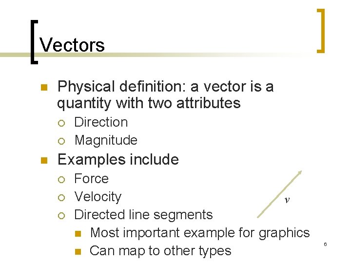
Vectors n Physical definition: a vector is a quantity with two attributes ¡ ¡ n Direction Magnitude Examples include ¡ ¡ ¡ Force Velocity v Directed line segments n Most important example for graphics n Can map to other types 6
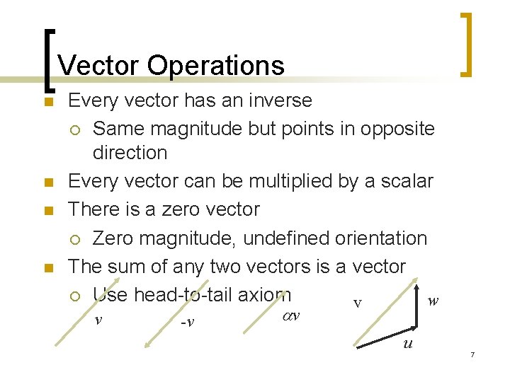
Vector Operations n n Every vector has an inverse ¡ Same magnitude but points in opposite direction Every vector can be multiplied by a scalar There is a zero vector ¡ Zero magnitude, undefined orientation The sum of any two vectors is a vector ¡ Use head-to-tail axiom w v v -v v u 7

Linear Vector Spaces n n n Mathematical system for manipulating vectors Operations ¡ Scalar-vector multiplication u= v ¡ Vector-vector addition: w=u+v Expressions such as v=u+2 w-3 r Make sense in a vector space 8
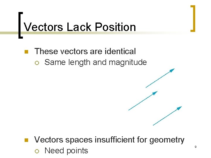
Vectors Lack Position n These vectors are identical ¡ Same length and magnitude n Vectors spaces insufficient for geometry ¡ Need points 9
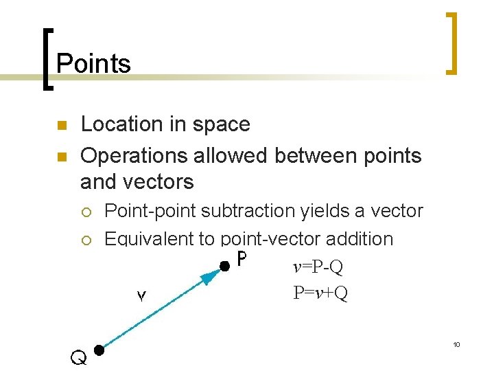
Points n n Location in space Operations allowed between points and vectors ¡ ¡ Point-point subtraction yields a vector Equivalent to point-vector addition v=P-Q P=v+Q 10
Affine Spaces n n Point + a vector space Operations Vector-vector addition ¡ Scalar-vector multiplication ¡ Point-vector addition ¡ Scalar-scalar operations For any point define ¡ 1 • P=P ¡ 0 • P = 0 (zero vector) ¡ n 11

Lines n Consider all points of the form ¡ ¡ P( )=P 0 + d Set of all points that pass through P 0 in the direction of the vector d 12
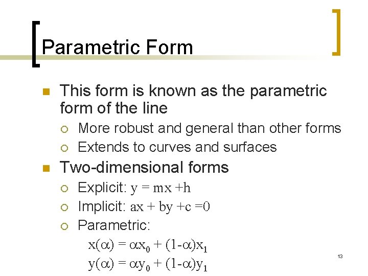
Parametric Form n This form is known as the parametric form of the line ¡ ¡ n More robust and general than other forms Extends to curves and surfaces Two-dimensional forms ¡ ¡ ¡ Explicit: y = mx +h Implicit: ax + by +c =0 Parametric: x( ) = x 0 + (1 - )x 1 y( ) = y 0 + (1 - )y 1 13
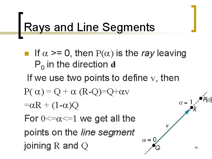
Rays and Line Segments If >= 0, then P( ) is the ray leaving P 0 in the direction d If we use two points to define v, then P( ) = Q + (R-Q)=Q+ v = R + (1 - )Q For 0<= <=1 we get all the points on the line segment joining R and Q n 14
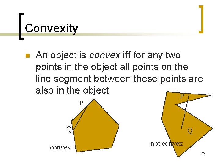
Convexity n An object is convex iff for any two points in the object all points on the line segment between these points are also in the object P P Q convex Q not convex 15
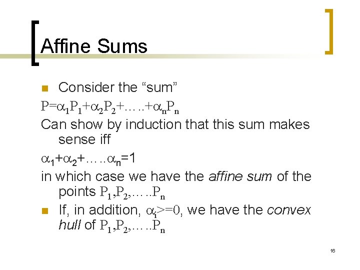
Affine Sums Consider the “sum” P= 1 P 1+ 2 P 2+…. . + n. Pn Can show by induction that this sum makes sense iff 1+ 2+…. . n=1 in which case we have the affine sum of the points P 1, P 2, …. . Pn n If, in addition, i>=0, we have the convex hull of P 1, P 2, …. . Pn n 16
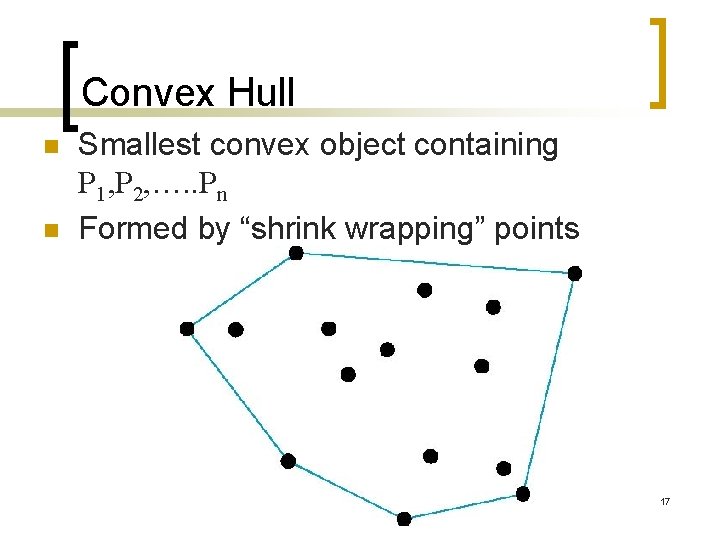
Convex Hull n n Smallest convex object containing P 1, P 2, …. . Pn Formed by “shrink wrapping” points 17
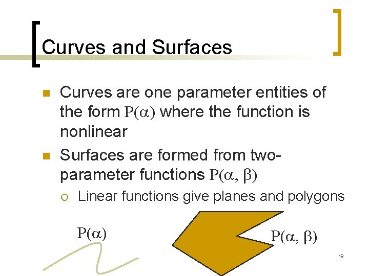
Curves and Surfaces n n Curves are one parameter entities of the form P( ) where the function is nonlinear Surfaces are formed from twoparameter functions P( , b) ¡ Linear functions give planes and polygons P( ) P( , b) 18
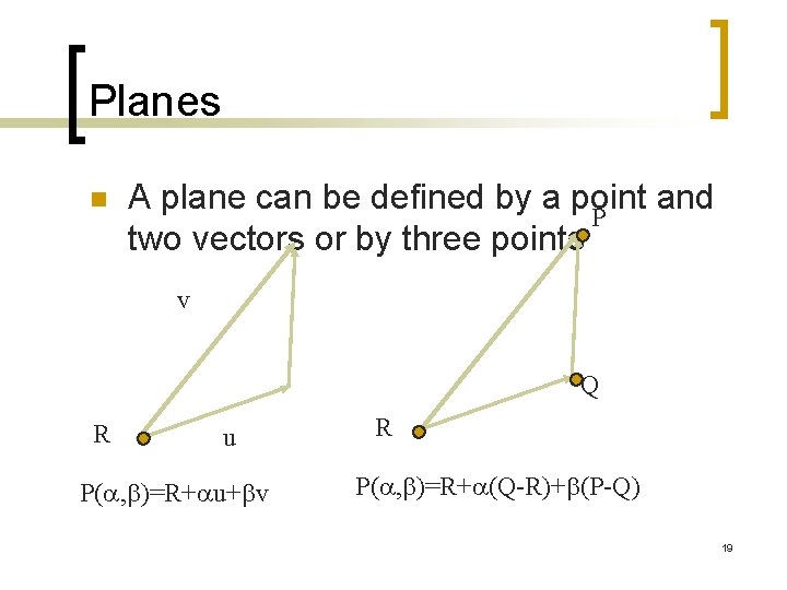
Planes n A plane can be defined by a point and P two vectors or by three points v Q R u P( , b)=R+ u+bv R P( , b)=R+ (Q-R)+b(P-Q) 19
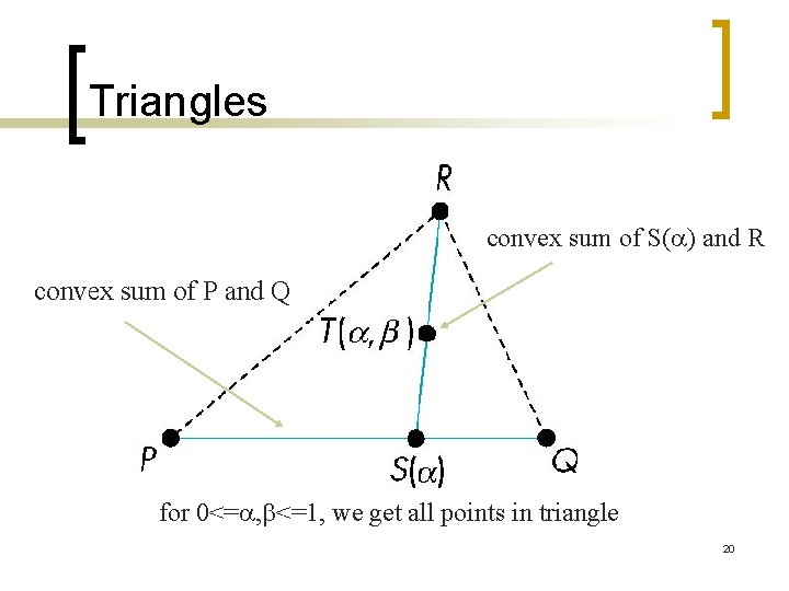
Triangles convex sum of S( ) and R convex sum of P and Q for 0<= , b<=1, we get all points in triangle 20
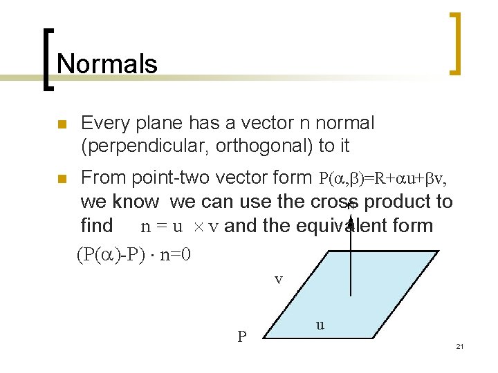
Normals n n Every plane has a vector n normal (perpendicular, orthogonal) to it From point-two vector form P( , b)=R+ u+bv, we know we can use the cross product to find n = u v and the equivalent form (P( )-P) n=0 v P u 21
Linear Independence n n n A set of vectors v 1, v 2, …, vn is linearly independent if 1 v 1+ 2 v 2+. . nvn=0 iff 1= 2=…=0 If a set of vectors is linearly independent, we cannot represent one in terms of the others If a set of vectors is linearly dependent, as least one can be written in terms of the others 22
Dimension In a vector space, the maximum number of linearly independent vectors is fixed and is called the dimension of the space n In an n-dimensional space, any set of n linearly independent vectors form a basis for the space n Given a basis v 1, v 2, …. , vn, any vector v can be written as v= 1 v 1+ 2 v 2 +…. + nvn where the { i} are unique n 23
Representation n n Until now we have been able to work with geometric entities without using any frame of reference, such as a coordinate system Need a frame of reference to relate points and objects to our physical world. ¡ ¡ ¡ For example, where is a point? Can’t answer without a reference system World coordinates Camera coordinates 24
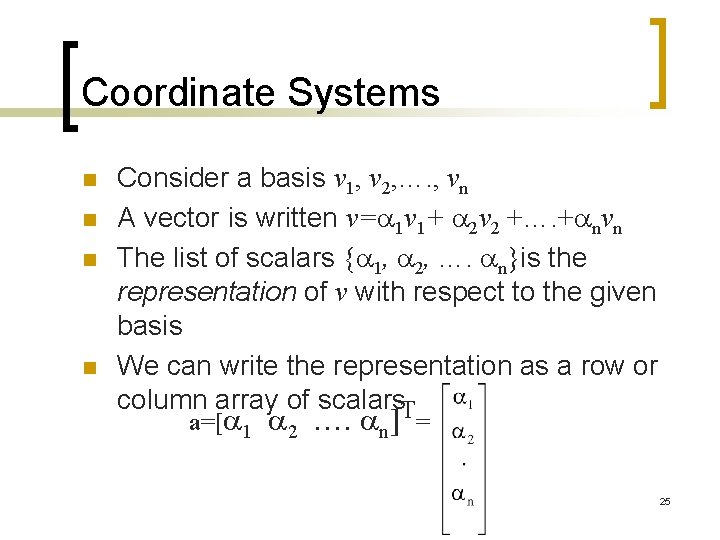
Coordinate Systems n n Consider a basis v 1, v 2, …. , vn A vector is written v= 1 v 1+ 2 v 2 +…. + nvn The list of scalars { 1, 2, …. n}is the representation of v with respect to the given basis We can write the representation as a row or column array of scalars. T a=[ 1 2 …. n] = 25
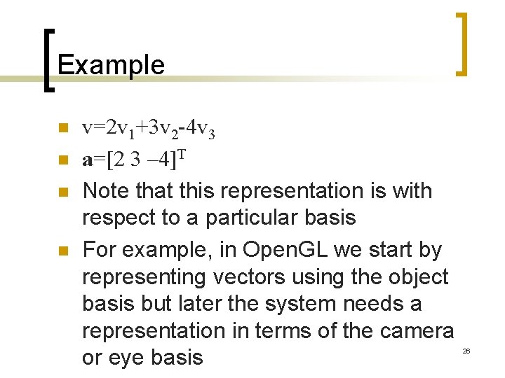
Example n n v=2 v 1+3 v 2 -4 v 3 a=[2 3 – 4]T Note that this representation is with respect to a particular basis For example, in Open. GL we start by representing vectors using the object basis but later the system needs a representation in terms of the camera or eye basis 26
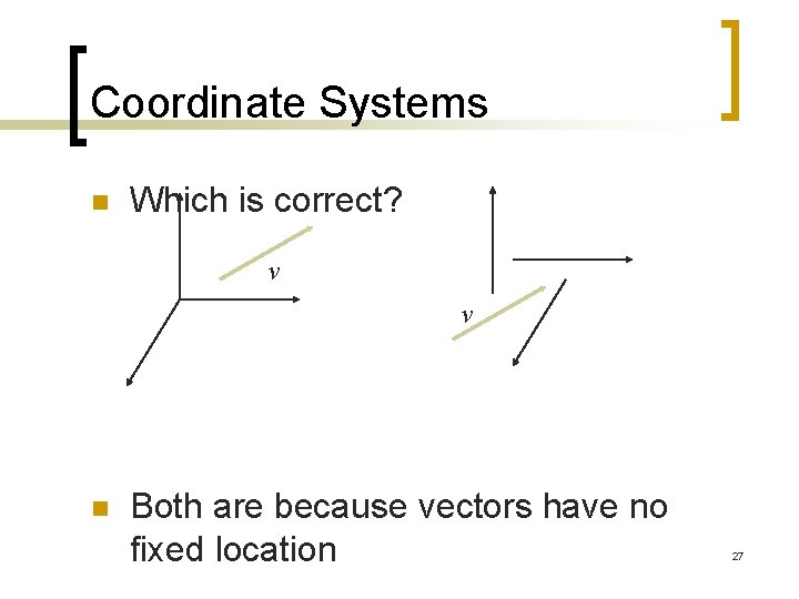
Coordinate Systems n Which is correct? v v n Both are because vectors have no fixed location 27
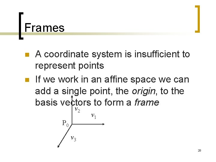
Frames n n A coordinate system is insufficient to represent points If we work in an affine space we can add a single point, the origin, to the basis vectors to form a frame v 2 P 0 v 1 v 3 28
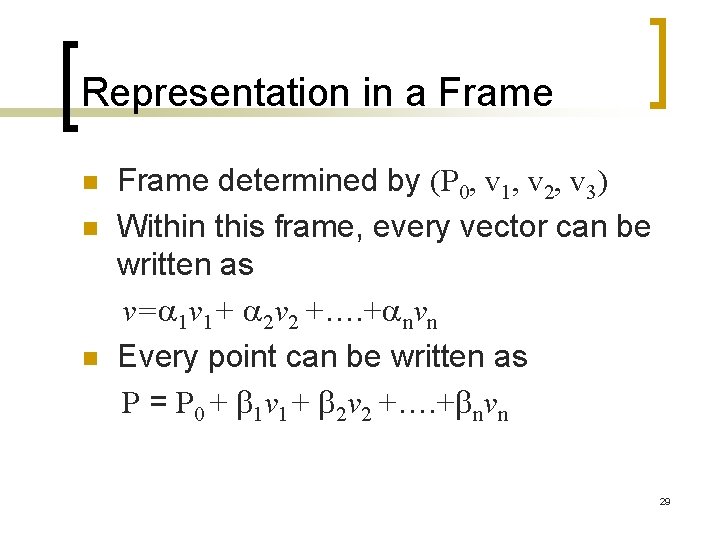
Representation in a Frame n n n Frame determined by (P 0, v 1, v 2, v 3) Within this frame, every vector can be written as v= 1 v 1+ 2 v 2 +…. + nvn Every point can be written as P = P 0 + b 1 v 1+ b 2 v 2 +…. +bnvn 29
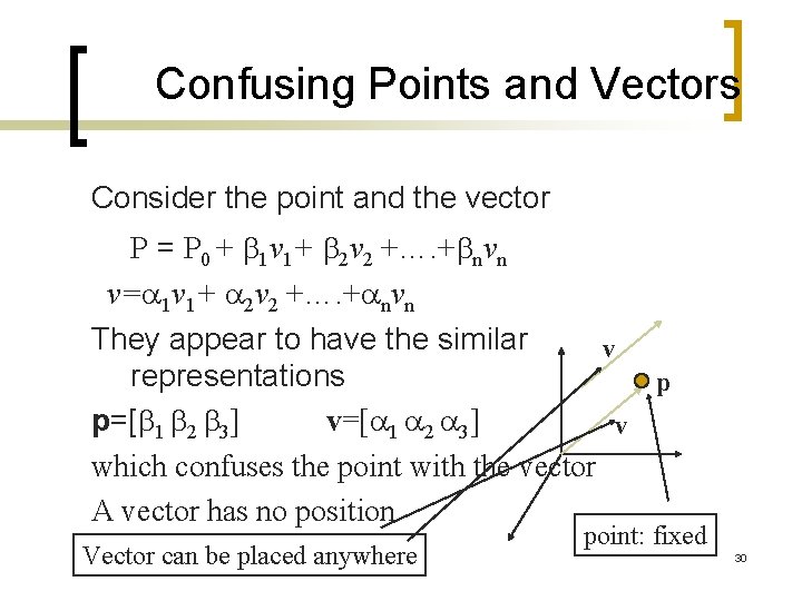
Confusing Points and Vectors Consider the point and the vector P = P 0 + b 1 v 1+ b 2 v 2 +…. +bnvn v= 1 v 1+ 2 v 2 +…. + nvn They appear to have the similar v representations p p=[b 1 b 2 b 3] v=[ 1 2 3] v which confuses the point with the vector A vector has no position Vector can be placed anywhere point: fixed 30
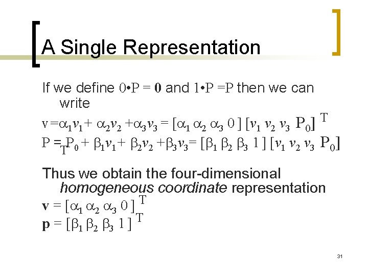
A Single Representation If we define 0 • P = 0 and 1 • P =P then we can write v= 1 v 1+ 2 v 2 + 3 v 3 = [ 1 2 3 0 ] [v 1 v 2 v 3 P 0] T P = P 0 + b 1 v 1+ b 2 v 2 +b 3 v 3= [b 1 b 2 b 3 1 ] [v 1 v 2 v 3 P 0] T Thus we obtain the four-dimensional homogeneous coordinate representation v = [ 1 2 3 0 ] T p = [b 1 b 2 b 3 1 ] T 31
![Homogeneous Coordinates The homogeneous coordinates form for a three dimensional point [x y z] Homogeneous Coordinates The homogeneous coordinates form for a three dimensional point [x y z]](http://slidetodoc.com/presentation_image_h2/2eeec72819cf6799713cfbd87af93872/image-32.jpg)
Homogeneous Coordinates The homogeneous coordinates form for a three dimensional point [x y z] is given as p =[x’ y’ z’ w] T =[wx wy wz w] T We return to a three dimensional point (for w 0) by x x’/w y y’/w z z’/w If w=0, the representation is that of a vector Note that homogeneous coordinates replaces points in three dimensions by lines through the origin in four dimensions For w=1, the representation of a point is [x y z 1] 32
Homogeneous Coordinates and Computer Graphics n Homogeneous coordinates are key to all computer graphics systems ¡ ¡ ¡ All standard transformations (rotation, translation, scaling) can be implemented with matrix multiplications using 4 x 4 matrices Hardware pipeline works with 4 dimensional representations For orthographic viewing, we can maintain w=0 for vectors and w=1 for points For perspective we need a perspective division 33 ¡
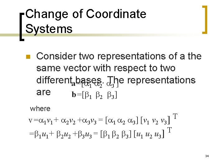
Change of Coordinate Systems n Consider two representations of a the same vector with respect to two differenta=[ bases. The representations ] 1 2 3 are b=[b 1 b 2 b 3] where v= 1 v 1+ 2 v 2 + 3 v 3 = [ 1 2 3] [v 1 v 2 v 3] T =b u +b u = [b b b ] [u u u ] T 1 1 2 2 3 3 1 2 3 34
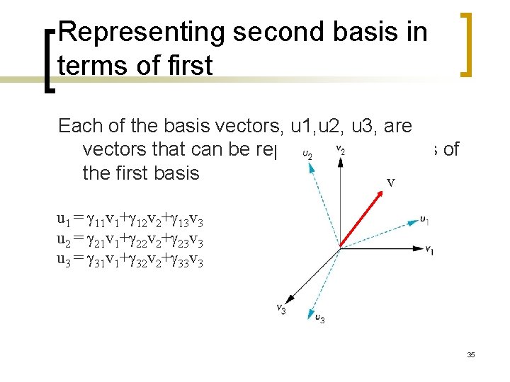
Representing second basis in terms of first Each of the basis vectors, u 1, u 2, u 3, are vectors that can be represented in terms of the first basis v u 1 = g 11 v 1+g 12 v 2+g 13 v 3 u 2 = g 21 v 1+g 22 v 2+g 23 v 3 u 3 = g 31 v 1+g 32 v 2+g 33 v 3 35
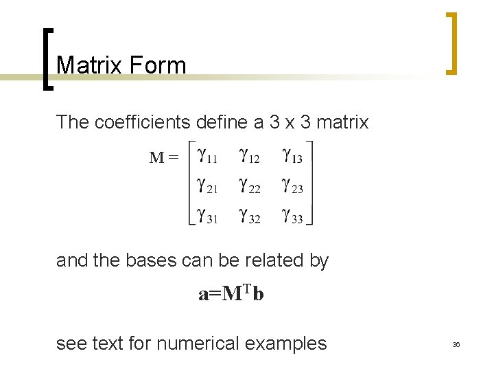
Matrix Form The coefficients define a 3 x 3 matrix M= and the bases can be related by a=MTb see text for numerical examples 36
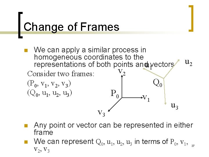
Change of Frames We can apply a similar process in homogeneous coordinates to the representations of both points andu 1 vectors v 2 Consider two frames: Q 0 (P 0, v 1, v 2, v 3) (Q 0, u 1, u 2, u 3) P 0 n v 1 v 3 n n u 2 u 3 Any point or vector can be represented in either frame We can represent Q 0, u 1, u 2, u 3 in terms of P 0, v 1, v 2, v 3 37
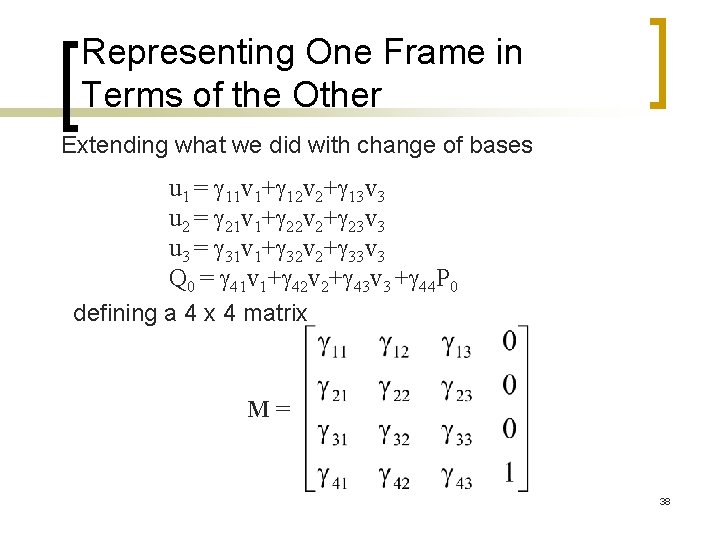
Representing One Frame in Terms of the Other Extending what we did with change of bases u 1 = g 11 v 1+g 12 v 2+g 13 v 3 u 2 = g 21 v 1+g 22 v 2+g 23 v 3 u 3 = g 31 v 1+g 32 v 2+g 33 v 3 Q 0 = g 41 v 1+g 42 v 2+g 43 v 3 +g 44 P 0 defining a 4 x 4 matrix M= 38
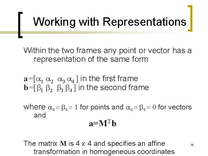
Working with Representations Within the two frames any point or vector has a representation of the same form a=[ 1 2 3 4 ] in the first frame b=[b 1 b 2 b 3 b 4 ] in the second frame where 4 = b 4 = 1 for points and 4 = b 4 = 0 for vectors and a=MTb The matrix M is 4 x 4 and specifies an affine transformation in homogeneous coordinates 39
Affine Transformations n n n Every linear transformation is equivalent to a change in frames Every affine transformation preserves lines However, an affine transformation has only 12 degrees of freedom because 4 of the elements in the matrix are fixed and are a subset of all possible 4 x 4 linear transformations 40
The World and Camera Frames n n n When we work with representations, we work with n-tuples or arrays of scalars Changes in frame are then defined by 4 x 4 matrices In Open. GL, the base frame that we start with is the world frame Eventually we represent entities in the camera frame by changing the world representation using the model-view matrix Initially these frames are the same (M=I) 41
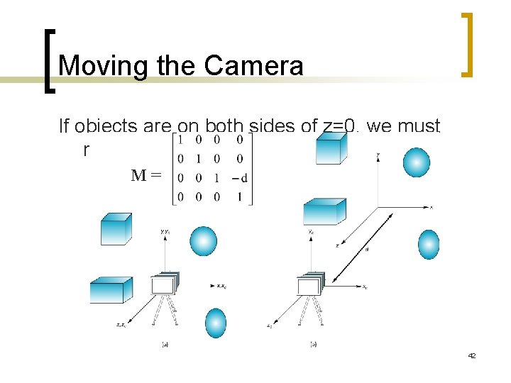
Moving the Camera If objects are on both sides of z=0, we must move camera frame M= 42
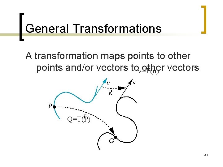
General Transformations A transformation maps points to other points and/or vectors tov=T(u) other vectors Q=T(P) 43
Affine Transformations n n Line preserving Characteristic of many physically important transformations ¡ ¡ n Rigid body transformations: rotation, translation Scaling, shear Importance in graphics is that we need only transform endpoints of line segments and let implementation draw line segment between the transformed endpoints 44
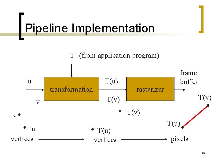
Pipeline Implementation T (from application program) u T(u) transformation v rasterizer T(v) v u vertices frame buffer T(u) vertices T(u) pixels 45
Notation We will be working with both coordinate-free representations of transformations and representations within a particular frame P, Q, R: points in an affine space u, v, w: vectors in an affine space , b, g: scalars p, q, r: representations of points -array of 4 scalars in homogeneous coordinates u, v, w: representations of points -array of 4 scalars in homogeneous coordinates 46
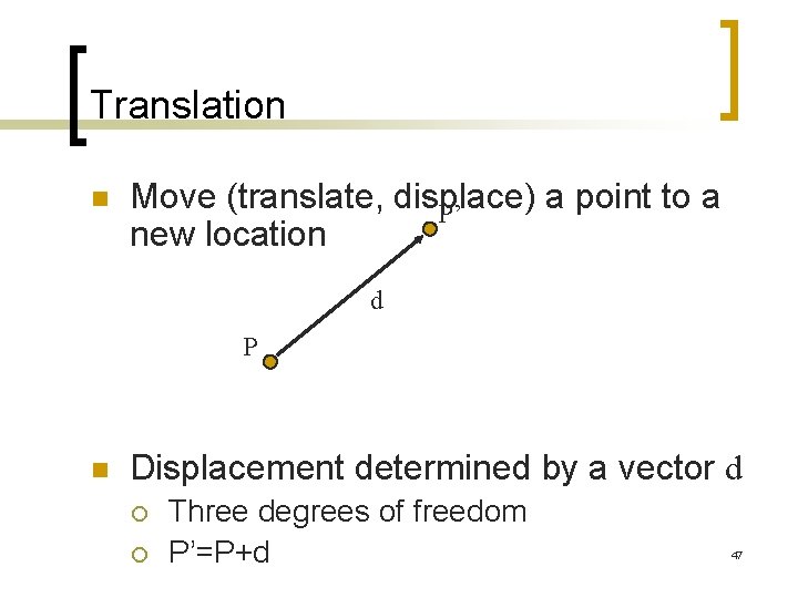
Translation n Move (translate, displace) a point to a P’ new location d P n Displacement determined by a vector d ¡ ¡ Three degrees of freedom P’=P+d 47
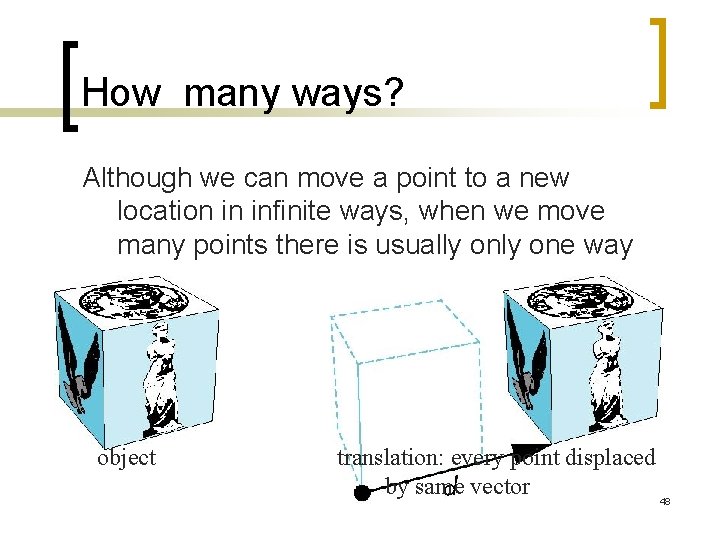
How many ways? Although we can move a point to a new location in infinite ways, when we move many points there is usually one way object translation: every point displaced by same vector 48
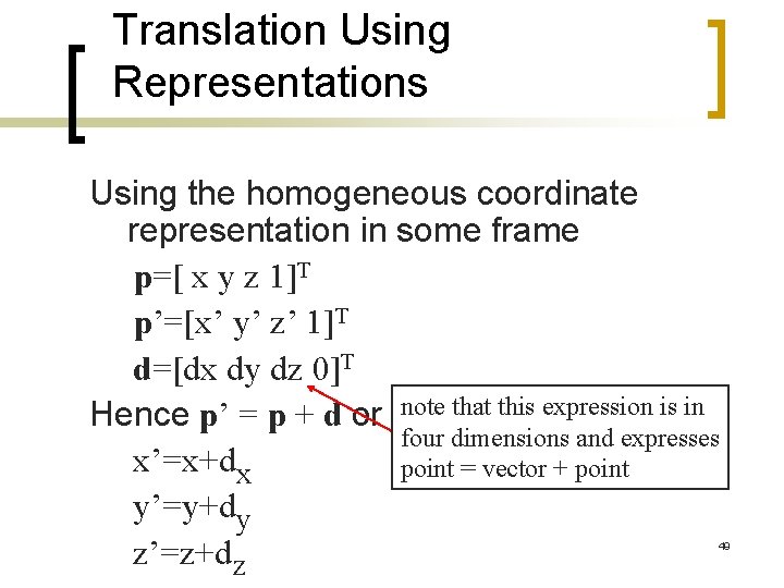
Translation Using Representations Using the homogeneous coordinate representation in some frame p=[ x y z 1]T p’=[x’ y’ z’ 1]T d=[dx dy dz 0]T Hence p’ = p + d or note that this expression is in four dimensions and expresses x’=x+dx point = vector + point y’=y+dy z’=z+dz 49

Translation Matrix We can also express translation using a 4 x 4 matrix T in homogeneous coordinates p’=Tp where T = T(dx, dy, dz) = This form is better for implementation because all affine transformations can be expressed this way and multiple transformations can be concatenated together 50
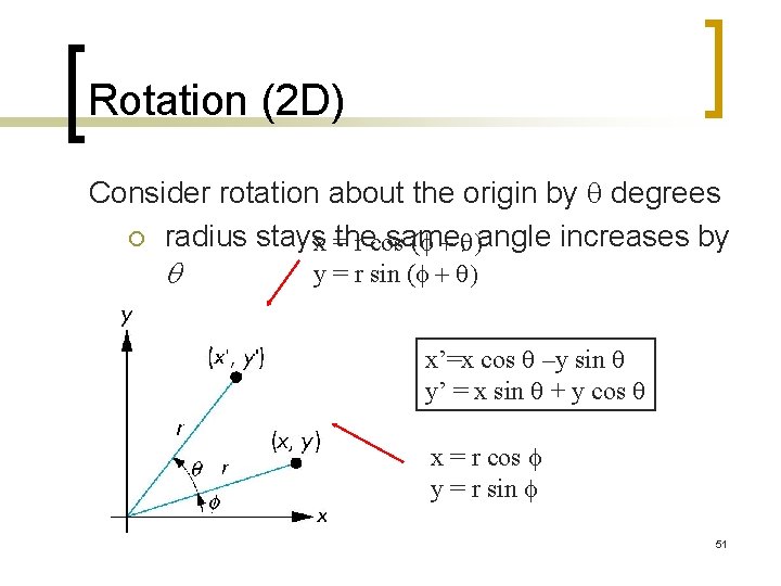
Rotation (2 D) Consider rotation about the origin by q degrees ¡ radius stays same, x =the r cos (f + q)angle increases by q y = r sin (f + q) x’=x cos q –y sin q y’ = x sin q + y cos q x = r cos f y = r sin f 51
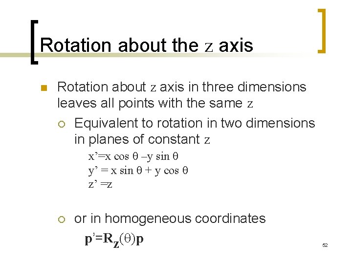
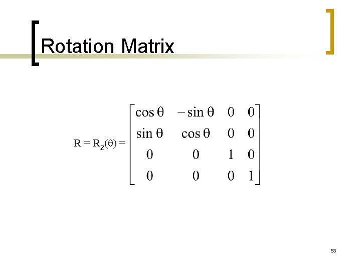
Rotation about the z axis n Rotation about z axis in three dimensions leaves all points with the same z ¡ Equivalent to rotation in two dimensions in planes of constant z x’=x cos q –y sin q y’ = x sin q + y cos q z’ =z ¡ or in homogeneous coordinates p’=Rz(q)p 52
Rotation Matrix R = Rz(q) = 53
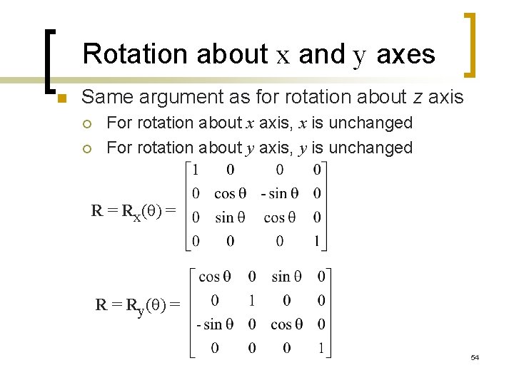
Rotation about x and y axes n Same argument as for rotation about z axis ¡ ¡ For rotation about x axis, x is unchanged For rotation about y axis, y is unchanged R = Rx(q) = Ry(q) = 54
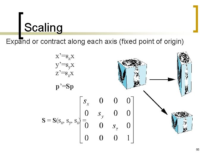
Scaling Expand or contract along each axis (fixed point of origin) x’=sxx y’=syx z’=szx p’=Sp S = S(sx, sy, sz) = 55
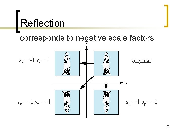
Reflection corresponds to negative scale factors sx = -1 sy = 1 original sx = -1 sy = -1 sx = 1 sy = -1 56
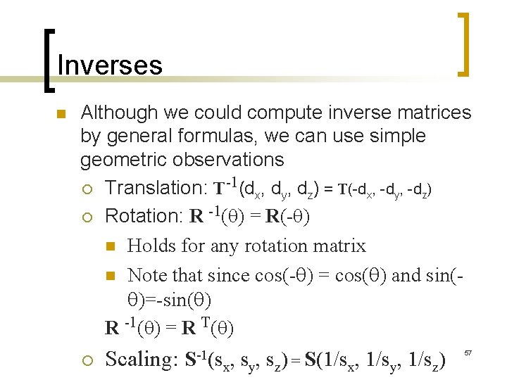
Inverses n Although we could compute inverse matrices by general formulas, we can use simple geometric observations -1 ¡ Translation: T (dx, dy, dz) = T(-dx, -dy, -dz) -1 ¡ Rotation: R (q) = R(-q) n Holds for any rotation matrix n Note that since cos(-q) = cos(q) and sin(q)=-sin(q) R -1(q) = R T(q) ¡ Scaling: S-1(s x, sy, sz) = S(1/sx, 1/sy, 1/sz) 57
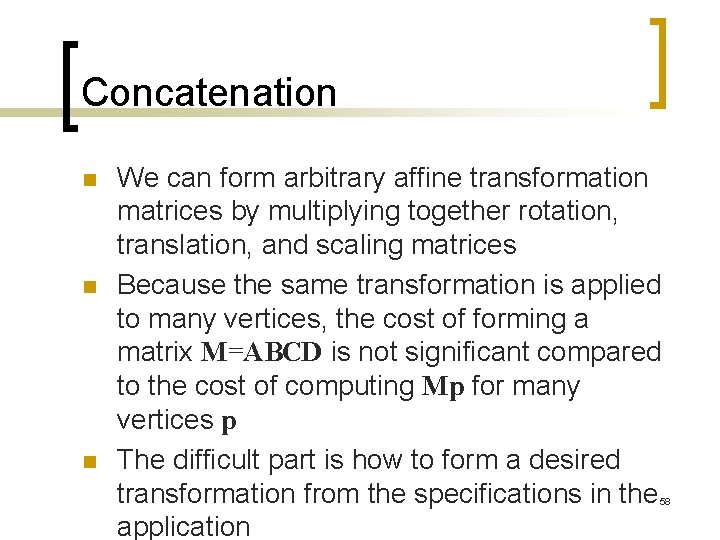
Concatenation n We can form arbitrary affine transformation matrices by multiplying together rotation, translation, and scaling matrices Because the same transformation is applied to many vertices, the cost of forming a matrix M=ABCD is not significant compared to the cost of computing Mp for many vertices p The difficult part is how to form a desired transformation from the specifications in the application 58
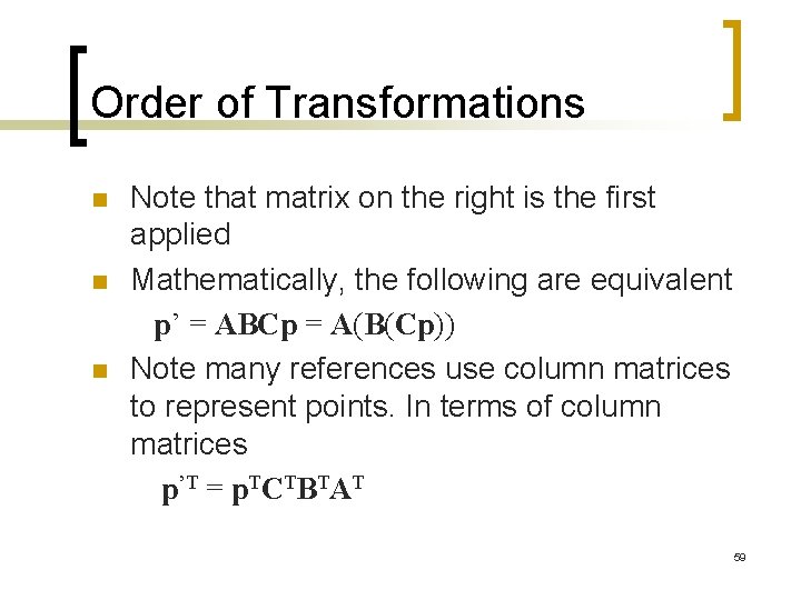
Order of Transformations n n n Note that matrix on the right is the first applied Mathematically, the following are equivalent p’ = ABCp = A(B(Cp)) Note many references use column matrices to represent points. In terms of column matrices p’T = p. TCTBTAT 59
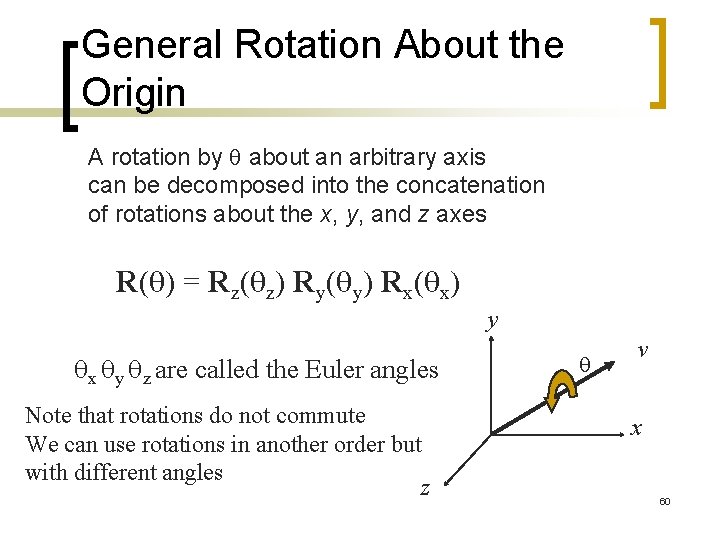
General Rotation About the Origin A rotation by q about an arbitrary axis can be decomposed into the concatenation of rotations about the x, y, and z axes R(q) = Rz(qz) Ry(qy) Rx(qx) y qx qy qz are called the Euler angles Note that rotations do not commute We can use rotations in another order but with different angles q v x z 60
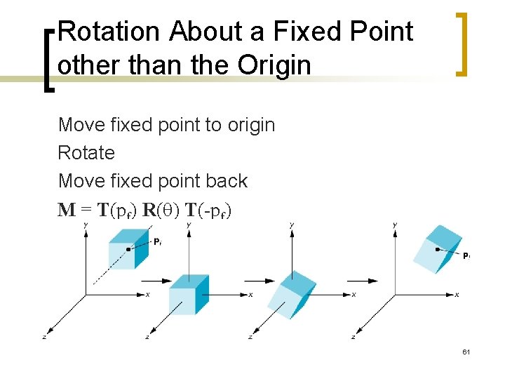
Rotation About a Fixed Point other than the Origin Move fixed point to origin Rotate Move fixed point back M = T(pf) R(q) T(-pf) 61
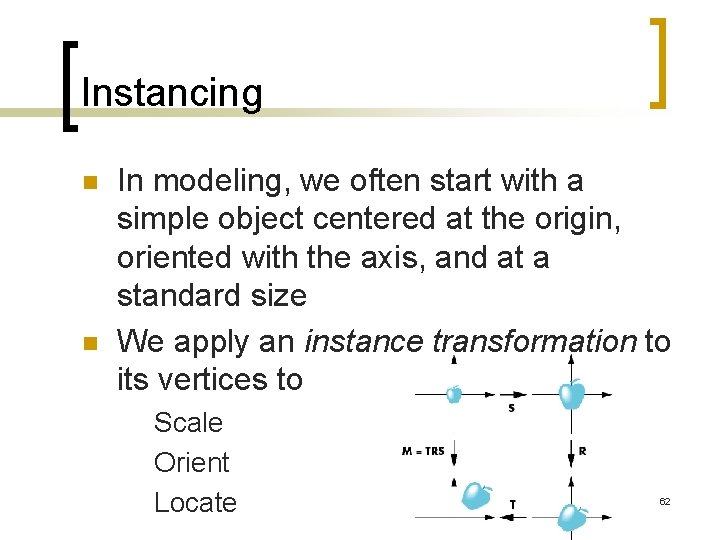
Instancing n n In modeling, we often start with a simple object centered at the origin, oriented with the axis, and at a standard size We apply an instance transformation to its vertices to Scale Orient Locate 62
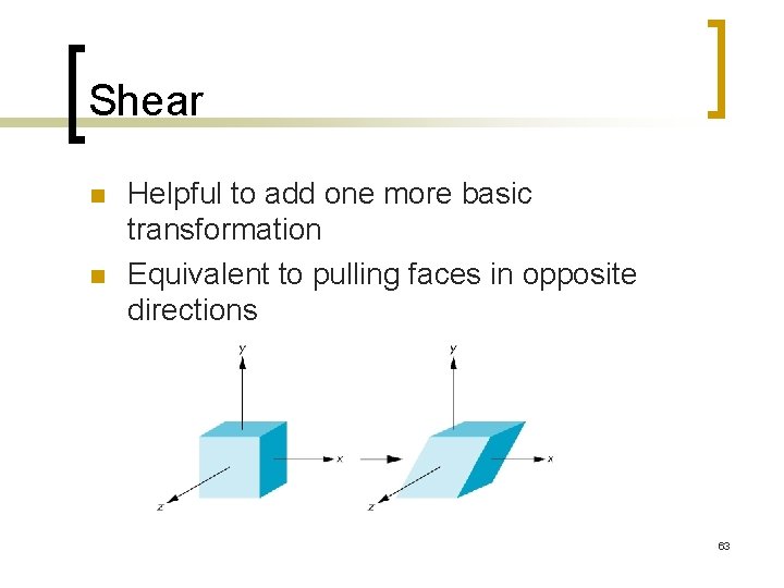
Shear n n Helpful to add one more basic transformation Equivalent to pulling faces in opposite directions 63
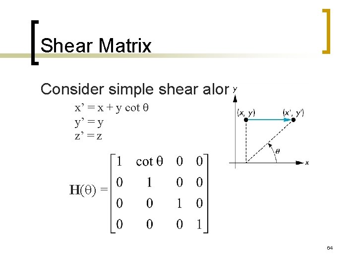
Shear Matrix Consider simple shear along x axis x’ = x + y cot q y’ = y z’ = z H(q) = 64
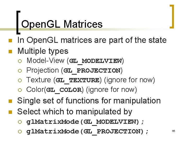
Open. GL Matrices n n In Open. GL matrices are part of the state Multiple types ¡ ¡ n n Model-View (GL_MODELVIEW) Projection (GL_PROJECTION) Texture (GL_TEXTURE) (ignore for now) Color(GL_COLOR) (ignore for now) Single set of functions for manipulation Select which to manipulated by ¡ ¡ gl. Matrix. Mode(GL_MODELVIEW); gl. Matrix. Mode(GL_PROJECTION); 65
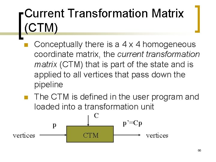
Current Transformation Matrix (CTM) n n Conceptually there is a 4 x 4 homogeneous coordinate matrix, the current transformation matrix (CTM) that is part of the state and is applied to all vertices that pass down the pipeline The CTM is defined in the user program and loaded into a transformation unit C p vertices CTM p’=Cp vertices 66
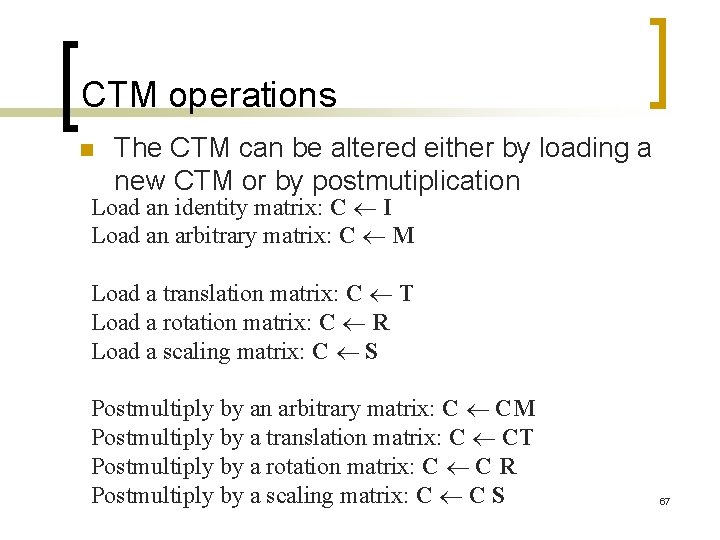
CTM operations n The CTM can be altered either by loading a new CTM or by postmutiplication Load an identity matrix: C I Load an arbitrary matrix: C M Load a translation matrix: C T Load a rotation matrix: C R Load a scaling matrix: C S Postmultiply by an arbitrary matrix: C CM Postmultiply by a translation matrix: C CT Postmultiply by a rotation matrix: C C R Postmultiply by a scaling matrix: C C S 67
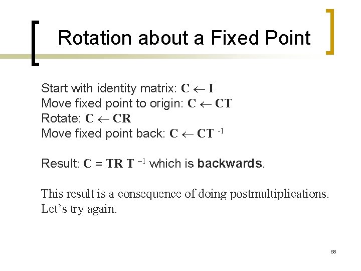
Rotation about a Fixed Point Start with identity matrix: C I Move fixed point to origin: C CT Rotate: C CR Move fixed point back: C CT -1 Result: C = TR T – 1 which is backwards. This result is a consequence of doing postmultiplications. Let’s try again. 68
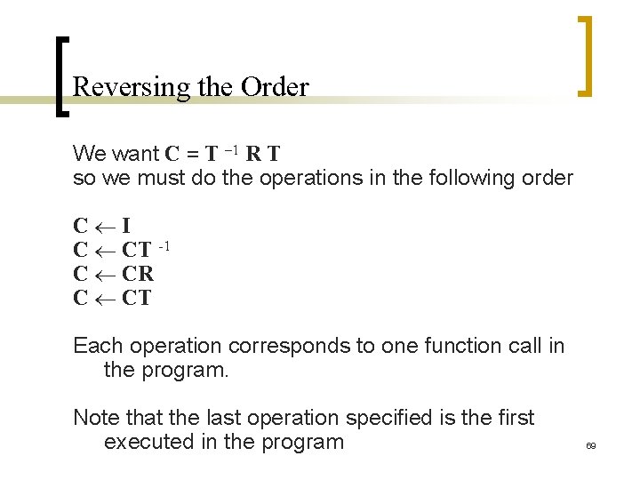
Reversing the Order We want C = T – 1 R T so we must do the operations in the following order C I C CT -1 C CR C CT Each operation corresponds to one function call in the program. Note that the last operation specified is the first executed in the program 69

CTM in Open. GL n n Open. GL has a model-view and a projection matrix in the pipeline which are concatenated together to form the CTM Can manipulate each by first setting the correct matrix mode 70
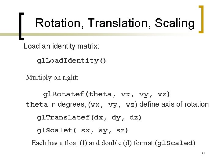
Rotation, Translation, Scaling Load an identity matrix: gl. Load. Identity() Multiply on right: gl. Rotatef(theta, vx, vy, vz) theta in degrees, (vx, vy, vz) define axis of rotation gl. Translatef(dx, dy, dz) gl. Scalef( sx, sy, sz) Each has a float (f) and double (d) format (gl. Scaled) 71
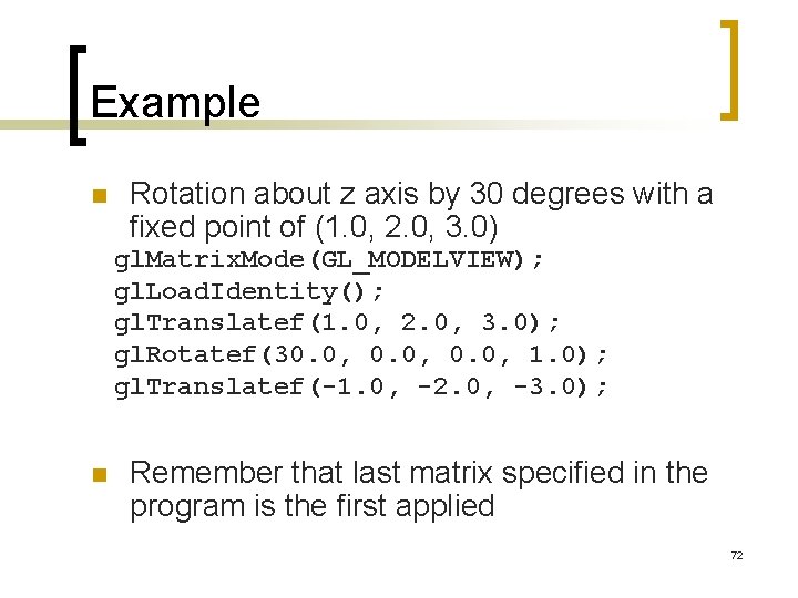
Example n Rotation about z axis by 30 degrees with a fixed point of (1. 0, 2. 0, 3. 0) gl. Matrix. Mode(GL_MODELVIEW); gl. Load. Identity(); gl. Translatef(1. 0, 2. 0, 3. 0); gl. Rotatef(30. 0, 1. 0); gl. Translatef(-1. 0, -2. 0, -3. 0); n Remember that last matrix specified in the program is the first applied 72
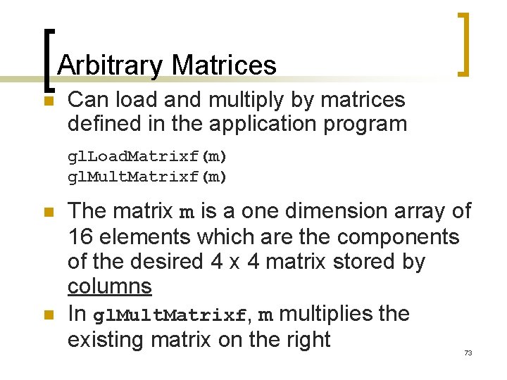
Arbitrary Matrices n Can load and multiply by matrices defined in the application program gl. Load. Matrixf(m) gl. Mult. Matrixf(m) n n The matrix m is a one dimension array of 16 elements which are the components of the desired 4 x 4 matrix stored by columns In gl. Mult. Matrixf, m multiplies the existing matrix on the right 73

Matrix Stacks n In many situations we want to save transformation matrices for use later ¡ ¡ n Traversing hierarchical data structures (Chapter 10) Avoiding state changes when executing display lists Open. GL maintains stacks for each type of matrix ¡ Access present type (as set by gl. Push. Matrix() gl. Matrix. Mode) by gl. Pop. Matrix() 74
Reading Back Matrices n Can also access matrices (and other parts of the state) by query functions gl. Get. Integerv gl. Get. Floatv gl. Get. Booleanv gl. Get. Doublev gl. Is. Enabled n For matrices, we use as double m[16]; gl. Get. Floatv(GL_MODELVIEW, m); 75
Using Transformations n Example: use idle function to rotate a cube and mouse function to change direction of rotation n Start with a program that draws a cube (colorcube. c) in a standard way ¡ Centered at origin ¡ Sides aligned with axes ¡ Will discuss modeling in next lecture 76
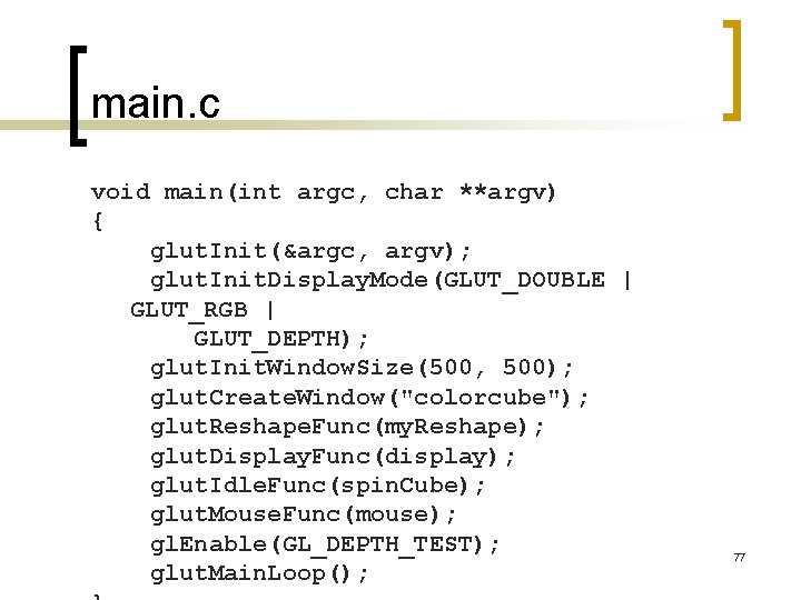
main. c void main(int argc, char **argv) { glut. Init(&argc, argv); glut. Init. Display. Mode(GLUT_DOUBLE | GLUT_RGB | GLUT_DEPTH); glut. Init. Window. Size(500, 500); glut. Create. Window("colorcube"); glut. Reshape. Func(my. Reshape); glut. Display. Func(display); glut. Idle. Func(spin. Cube); glut. Mouse. Func(mouse); gl. Enable(GL_DEPTH_TEST); glut. Main. Loop(); 77
![Idle and Mouse callbacks void spin. Cube() { theta[axis] += 2. 0; if( theta[axis] Idle and Mouse callbacks void spin. Cube() { theta[axis] += 2. 0; if( theta[axis]](http://slidetodoc.com/presentation_image_h2/2eeec72819cf6799713cfbd87af93872/image-78.jpg)
Idle and Mouse callbacks void spin. Cube() { theta[axis] += 2. 0; if( theta[axis] > 360. 0 ) theta[axis] -= 360. 0; void mouse(int btn, int state, int x, int y) glut. Post. Redisplay(); { }if(btn==GLUT_LEFT_BUTTON && state == GLUT_DOWN) axis = 0; if(btn==GLUT_MIDDLE_BUTTON && state == GLUT_DOWN) axis = 1; if(btn==GLUT_RIGHT_BUTTON && state == GLUT_DOWN) axis = 2; } 78
![Display callback void display() { gl. Clear(GL_COLOR_BUFFER_BIT | GL_DEPTH_BUFFER_BIT); gl. Load. Identity(); gl. Rotatef(theta[0], Display callback void display() { gl. Clear(GL_COLOR_BUFFER_BIT | GL_DEPTH_BUFFER_BIT); gl. Load. Identity(); gl. Rotatef(theta[0],](http://slidetodoc.com/presentation_image_h2/2eeec72819cf6799713cfbd87af93872/image-79.jpg)
Display callback void display() { gl. Clear(GL_COLOR_BUFFER_BIT | GL_DEPTH_BUFFER_BIT); gl. Load. Identity(); gl. Rotatef(theta[0], 1. 0, 0. 0); gl. Rotatef(theta[1], 0. 0, 1. 0, 0. 0); gl. Rotatef(theta[2], 0. 0, 1. 0); colorcube(); glut. Swap. Buffers(); } Note that because of fixed from of callbacks, variables such as theta and axis must be defined as globals Camera information is in standard reshape callback 79
Using the Model-view Matrix n In Open. GL the model-view matrix is used to ¡ Position the camera n Can be done by rotations and translations but is often easier to use glu. Look. At Build models of objects The projection matrix is used to define the view volume and to select a camera lens ¡ n 80
Model-view and Projection Matrices n Although both are manipulated by the same functions, we have to be careful because incremental changes are always made by postmultiplication ¡ For example, rotating model-view and projection matrices by the same matrix are not equivalent operations. Postmultiplication of the model-view matrix is equivalent to premultiplication of the projection matrix 81
Smooth Rotation n n From a practical standpoint, we are often want to use transformations to move and reorient an object smoothly ¡ Problem: find a sequence of model-view matrices M 0, M 1, …. . , Mn so that when they are applied successively to one or more objects we see a smooth transition For orientating an object, we can use the fact that every rotation corresponds to part of a great circle on a sphere ¡ Find the axis of rotation and angle ¡ Virtual trackball (see text) 82
Incremental Rotation n Consider the two approaches ¡ For a sequence of rotation matrices R 0, R 1, …. . , Rn , find the Euler angles for each and use Ri= Riz Riy Rix n Not very efficient ¡ Use the final positions to determine the axis and angle of rotation, then increment only the angle n Quaternions can be more efficient than either 83
Quaternions n n Extension of imaginary numbers from two to three dimensions Requires one real and three imaginary components i, j, k q=q 0+q 1 i+q 2 j+q 3 k n Quaternions can express rotations on sphere smoothly and efficiently. Process: ¡ ¡ ¡ Model-view matrix quaternion Carry out operations with quaternions Quaternion Model-view matrix 84
Interfaces n n n One of the major problems in interactive computer graphics is how to use twodimensional devices such as a mouse to interface with three dimensional obejcts Example: how to form an instance matrix? Some alternatives ¡ Virtual trackball ¡ 3 D input devices such as the spaceball ¡ Use areas of the screen n Distance from center controls angle, position, scale depending on mouse 85
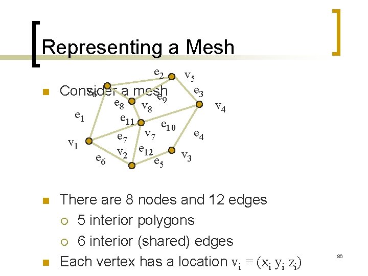
Representing a Mesh e 2 n v 6 Consider a mesh e e 1 v 1 n n e 6 v 5 e 3 e 8 v 9 v 4 8 e 11 e 10 e 4 e 7 v 2 e 12 e 5 v 3 There are 8 nodes and 12 edges ¡ 5 interior polygons ¡ 6 interior (shared) edges Each vertex has a location vi = (xi yi zi) 86
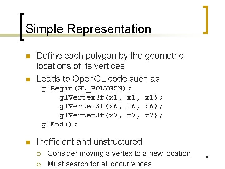
Simple Representation n n Define each polygon by the geometric locations of its vertices Leads to Open. GL code such as gl. Begin(GL_POLYGON); gl. Vertex 3 f(x 1, x 1); gl. Vertex 3 f(x 6, x 6); gl. Vertex 3 f(x 7, x 7); gl. End(); n Inefficient and unstructured ¡ ¡ Consider moving a vertex to a new location Must search for all occurrences 87
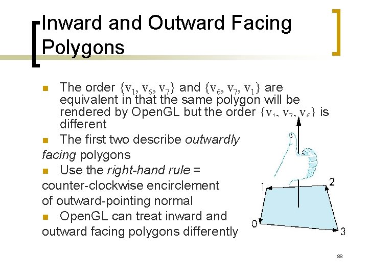
Inward and Outward Facing Polygons The order {v 1, v 6, v 7} and {v 6, v 7, v 1} are equivalent in that the same polygon will be rendered by Open. GL but the order {v 1, v 7, v 6} is different n The first two describe outwardly facing polygons n Use the right-hand rule = counter-clockwise encirclement of outward-pointing normal n Open. GL can treat inward and outward facing polygons differently n 88
Geometry vs Topology n Generally it is a good idea to look for data structures that separate the geometry from the topology ¡ ¡ ¡ Geometry: locations of the vertices Topology: organization of the vertices and edges Example: a polygon is an ordered list of vertices with an edge connecting successive pairs of vertices and the last to the first Topology holds even if geometry changes 89 ¡
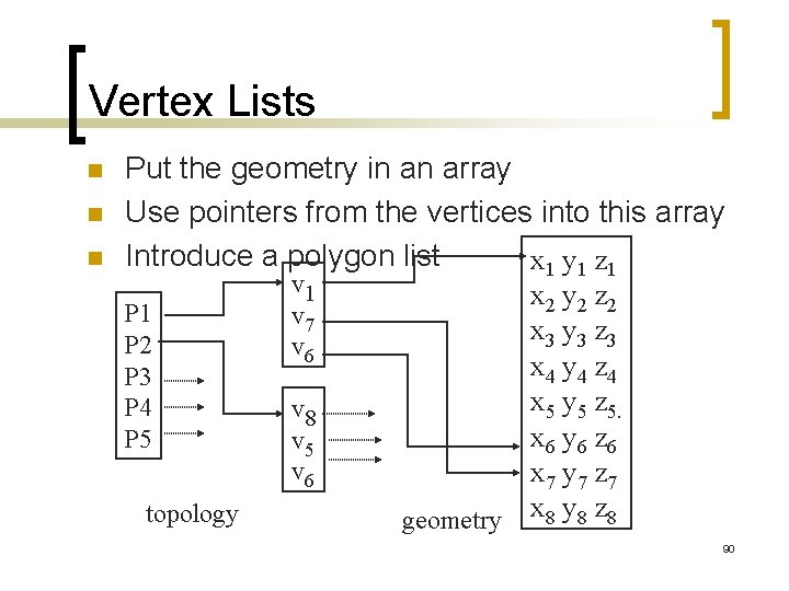
Vertex Lists n n n Put the geometry in an array Use pointers from the vertices into this array Introduce a polygon list x 1 y 1 z 1 v 1 x 2 y 2 z 2 P 1 v 7 x 3 y 3 z 3 P 2 v 6 x 4 y 4 z 4 P 3 x 5 y 5 z 5. P 4 v 8 x 6 y 6 z 6 P 5 v 6 x 7 y 7 z 7 topology geometry x 8 y 8 z 8 90
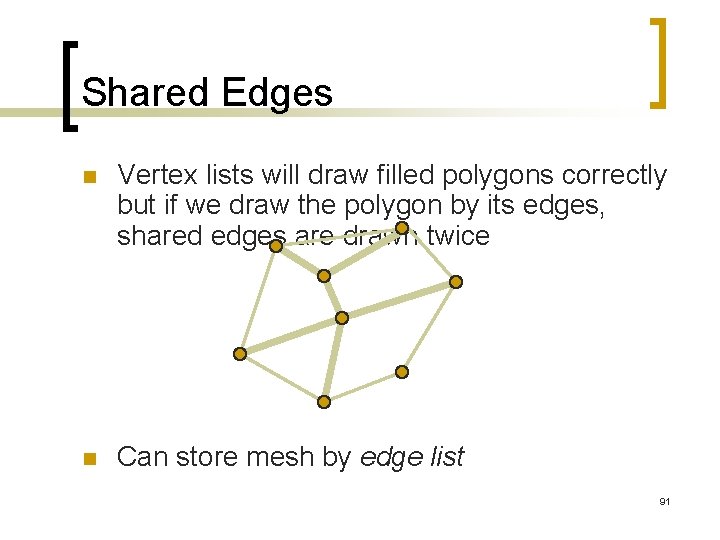
Shared Edges n Vertex lists will draw filled polygons correctly but if we draw the polygon by its edges, shared edges are drawn twice n Can store mesh by edge list 91
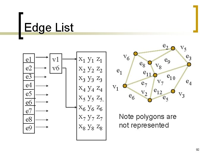
Edge List e 2 e 1 e 2 e 3 e 4 e 5 e 6 e 7 e 8 e 9 v 1 v 6 x 1 y 1 z 1 x 2 y 2 z 2 x 3 y 3 z 3 x 4 y 4 z 4 x 5 y 5 z 5. x 6 y 6 z 6 x 7 y 7 z 7 x 8 y 8 z 8 v 6 e 1 v 1 e 6 v 5 e 3 e 8 v e 9 8 e 11 e 10 e 4 e 7 v 2 e 12 e 5 v 3 Note polygons are not represented 92
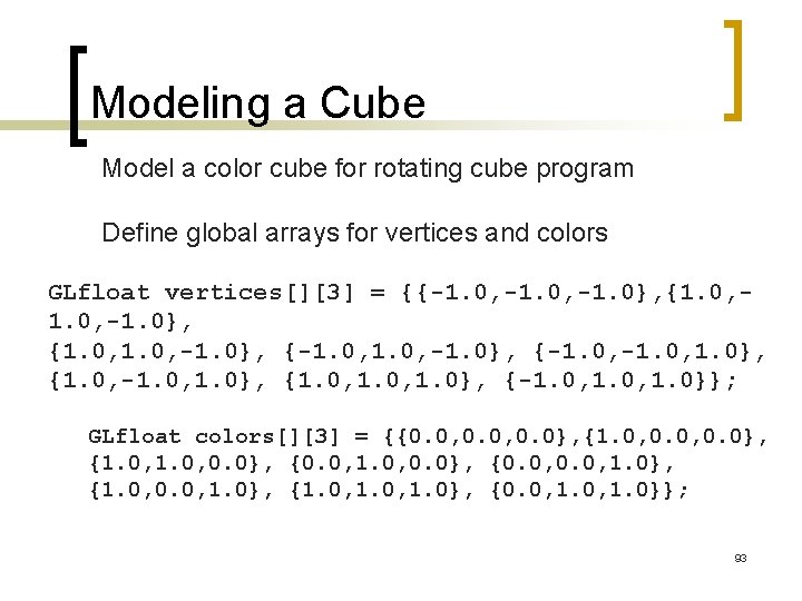
Modeling a Cube Model a color cube for rotating cube program Define global arrays for vertices and colors GLfloat vertices[][3] = {{-1. 0, -1. 0}, {1. 0, -1. 0}, {-1. 0, 1. 0}, {1. 0, 1. 0}, {-1. 0, 1. 0}}; GLfloat colors[][3] = {{0. 0, 0. 0}, {1. 0, 0. 0}, {0. 0, 1. 0}, {1. 0, 1. 0}, {0. 0, 1. 0}}; 93
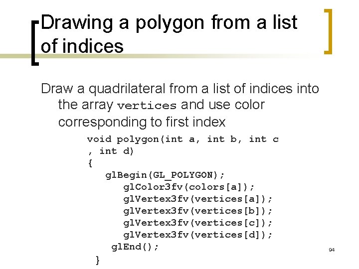
Drawing a polygon from a list of indices Draw a quadrilateral from a list of indices into the array vertices and use color corresponding to first index void polygon(int a, int b, int c , int d) { gl. Begin(GL_POLYGON); gl. Color 3 fv(colors[a]); gl. Vertex 3 fv(vertices[b]); gl. Vertex 3 fv(vertices[c]); gl. Vertex 3 fv(vertices[d]); gl. End(); } 94
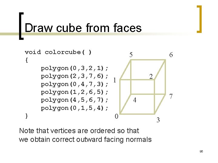
Draw cube from faces void colorcube( ) { polygon(0, 3, 2, 1); polygon(2, 3, 7, 6); 1 polygon(0, 4, 7, 3); polygon(1, 2, 6, 5); polygon(4, 5, 6, 7); polygon(0, 1, 5, 4); } 0 5 6 2 7 4 3 Note that vertices are ordered so that we obtain correct outward facing normals 95
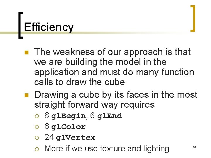
Efficiency n n The weakness of our approach is that we are building the model in the application and must do many function calls to draw the cube Drawing a cube by its faces in the most straight forward way requires ¡ ¡ 6 gl. Begin, 6 gl. End 6 gl. Color 24 gl. Vertex More if we use texture and lighting 96
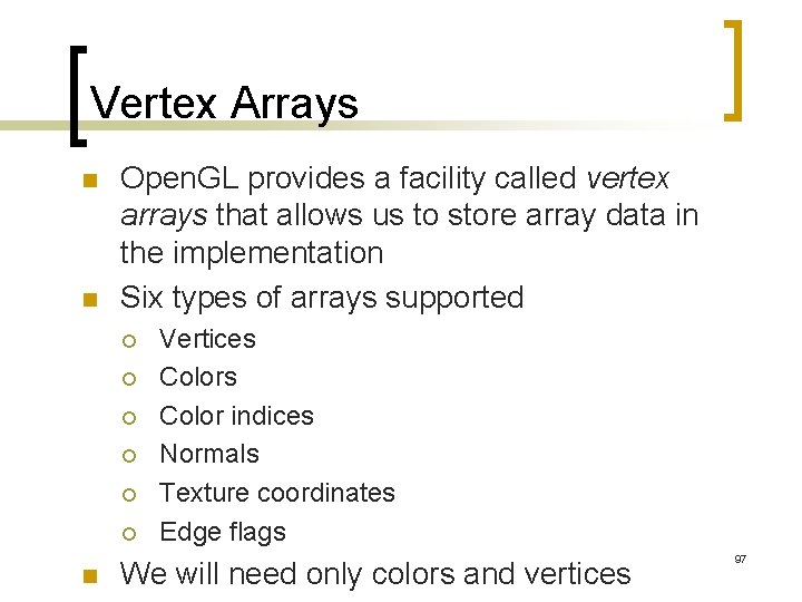
Vertex Arrays n n Open. GL provides a facility called vertex arrays that allows us to store array data in the implementation Six types of arrays supported ¡ ¡ ¡ n Vertices Color indices Normals Texture coordinates Edge flags We will need only colors and vertices 97
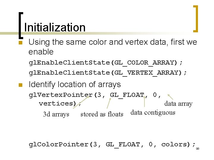
Initialization n Using the same color and vertex data, first we enable gl. Enable. Client. State(GL_COLOR_ARRAY); gl. Enable. Client. State(GL_VERTEX_ARRAY); n Identify location of arrays gl. Vertex. Pointer(3, GL_FLOAT, 0, vertices); data array 3 d arrays stored as floats data contiguous gl. Color. Pointer(3, GL_FLOAT, 0, colors); 98
![Mapping indices to faces n Form an array of face indices GLubyte cube. Indices[24] Mapping indices to faces n Form an array of face indices GLubyte cube. Indices[24]](http://slidetodoc.com/presentation_image_h2/2eeec72819cf6799713cfbd87af93872/image-99.jpg)
Mapping indices to faces n Form an array of face indices GLubyte cube. Indices[24] = {0, 3, 2, 1, 2, 3, 7, 6 0, 4, 7, 3, 1, 2, 6, 5, 4, 5, 6, 7, 0, 1, 5, 4}; n n Each successive four indices describe a face of the cube Draw through gl. Draw. Elements which replaces all gl. Vertex and gl. Color calls in the display callback 99
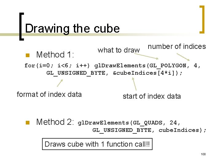
Drawing the cube n what to draw Method 1: number of indices for(i=0; i<6; i++) gl. Draw. Elements(GL_POLYGON, 4, GL_UNSIGNED_BYTE, &cube. Indices[4*i]); format of index data n Method 2: start of index data gl. Draw. Elements(GL_QUADS, 24, GL_UNSIGNED_BYTE, cube. Indices); Draws cube with 1 function call!! 100
- Slides: 100