Chapter 4 Fundamental statistical characteristics II Dispersion and

Chapter 4 Fundamental statistical characteristics II: Dispersion and form measurements

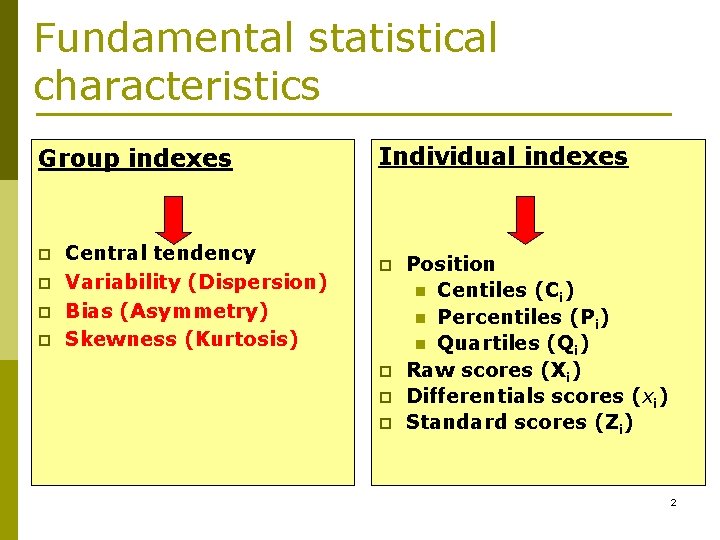
Fundamental statistical characteristics Group indexes p p Central tendency Variability (Dispersion) Bias (Asymmetry) Skewness (Kurtosis) Individual indexes p p Position n Centiles (Ci) n Percentiles (Pi) n Quartiles (Qi) Raw scores (Xi) Differentials scores (xi) Standard scores (Zi) 2

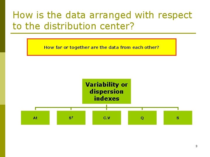
How is the data arranged with respect to the distribution center? How far or together are the data from each other? Variability or dispersion indexes At S 2 C. V Q S 3

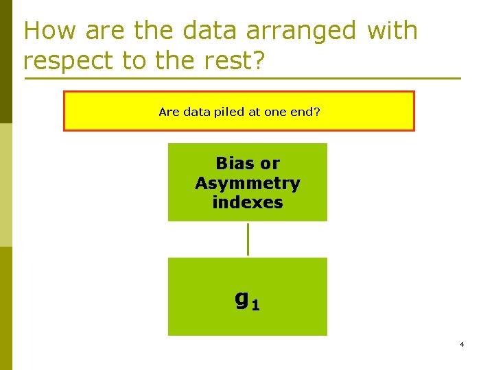
How are the data arranged with respect to the rest? Are data piled at one end? Bias or Asymmetry indexes g 1 4

Which form is the distribution? Is it flattened or sharp? Skewness or Kurtosis indexes g 2 5

Variability or dispersion indexes 6

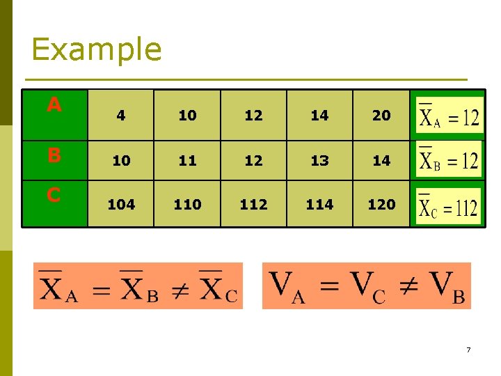
Example A 4 10 12 14 20 B 10 11 12 13 14 C 104 110 112 114 120 7

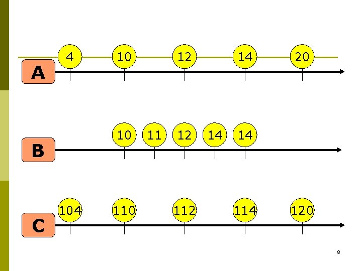
A 4 10 B C 10 104 110 12 112 14 14 20 14 120 8

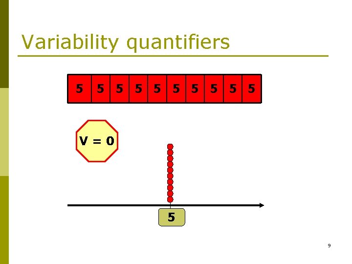
Variability quantifiers 5 5 5 5 5 V=0 5 9

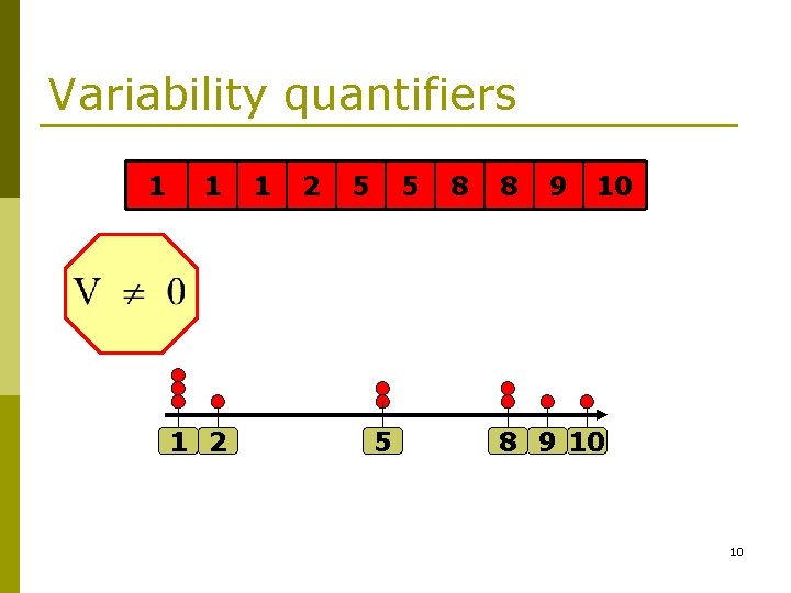
Variability quantifiers 1 1 1 2 5 5 5 8 8 9 10 10

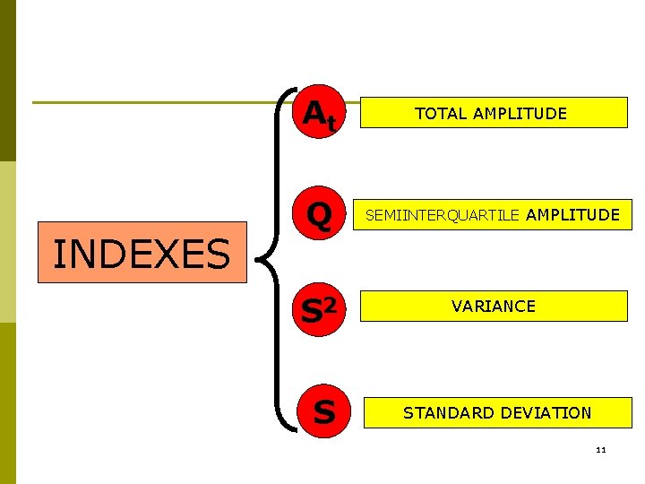
INDEXES At TOTAL AMPLITUDE Q SEMIINTERQUARTILE AMPLITUDE S 2 VARIANCE S STANDARD DEVIATION 11

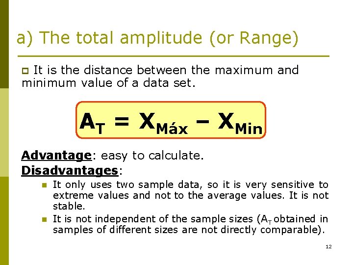
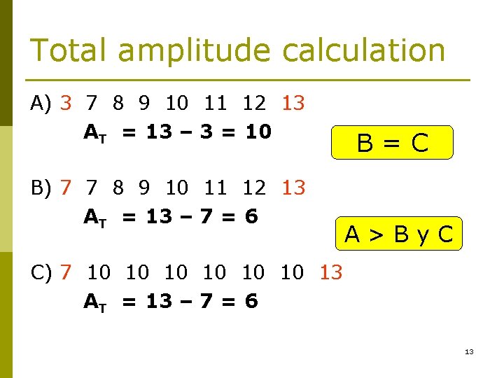
a) The total amplitude (or Range) It is the distance between the maximum and minimum value of a data set. p AT = XMáx – XMin Advantage: easy to calculate. Disadvantages: n n It only uses two sample data, so it is very sensitive to extreme values and not to the average values. It is not stable. It is not independent of the sample sizes (AT obtained in samples of different sizes are not directly comparable). 12

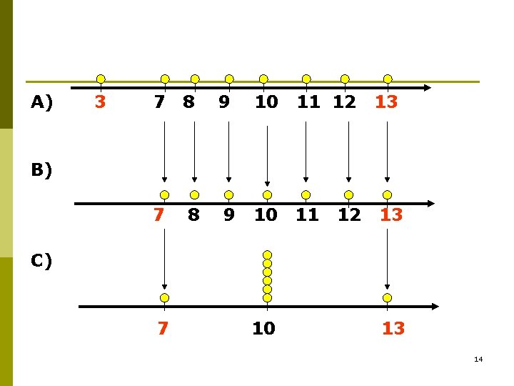
Total amplitude calculation A) 3 7 8 9 10 11 12 13 AT = 13 – 3 = 10 B) 7 7 8 9 10 11 12 13 AT = 13 – 7 = 6 B=C A>By. C C) 7 10 10 10 13 AT = 13 – 7 = 6 13

A) 3 7 8 9 10 11 12 13 7 8 9 10 11 13 B) 12 C) 7 10 13 14

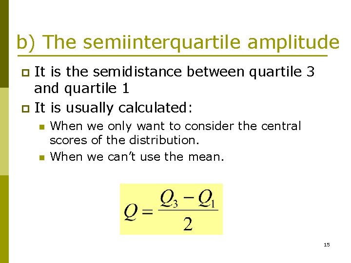
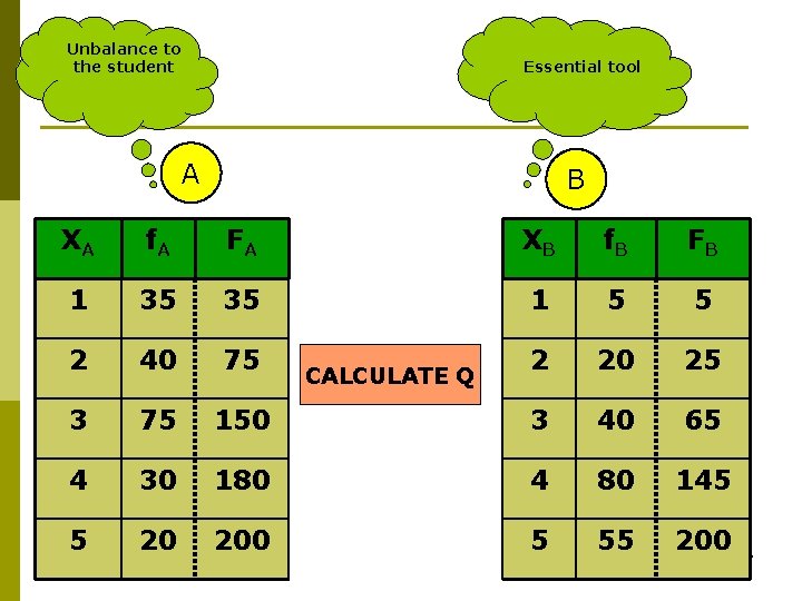
b) The semiinterquartile amplitude It is the semidistance between quartile 3 and quartile 1 p It is usually calculated: p n n When we only want to consider the central scores of the distribution. When we can’t use the mean. 15

Calculation example Data analysis: A) Unbalance to the student of Psychology. B) It is an essential tool for Psychology. 16

Unbalance to the student Essential tool A B XA f. A FA XB f. B FB 1 35 35 1 5 5 2 40 75 2 20 25 3 75 150 3 40 65 4 30 180 4 80 145 5 20 200 5 55 200 CALCULATE Q 17

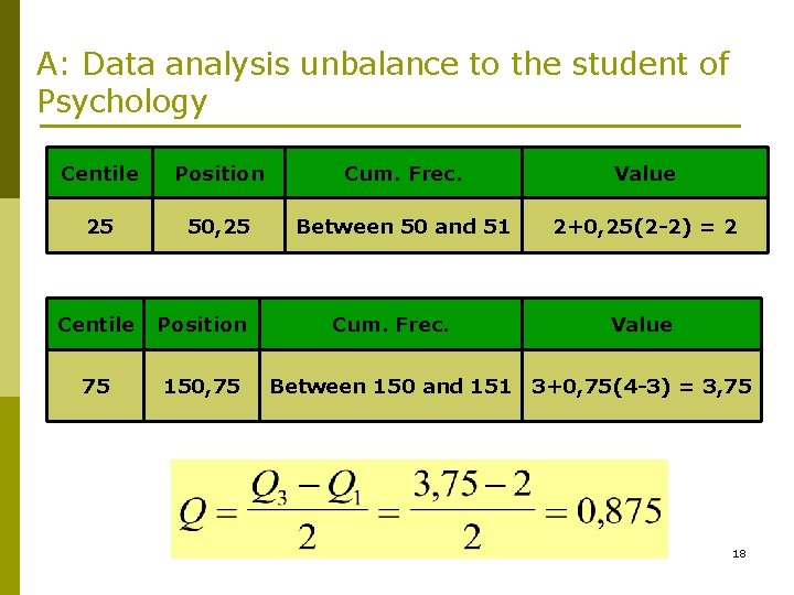
A: Data analysis unbalance to the student of Psychology Centile Position Cum. Frec. Value 25 50, 25 Between 50 and 51 2+0, 25(2 -2) = 2 Centile Position 75 150, 75 Cum. Frec. Value Between 150 and 151 3+0, 75(4 -3) = 3, 75 18

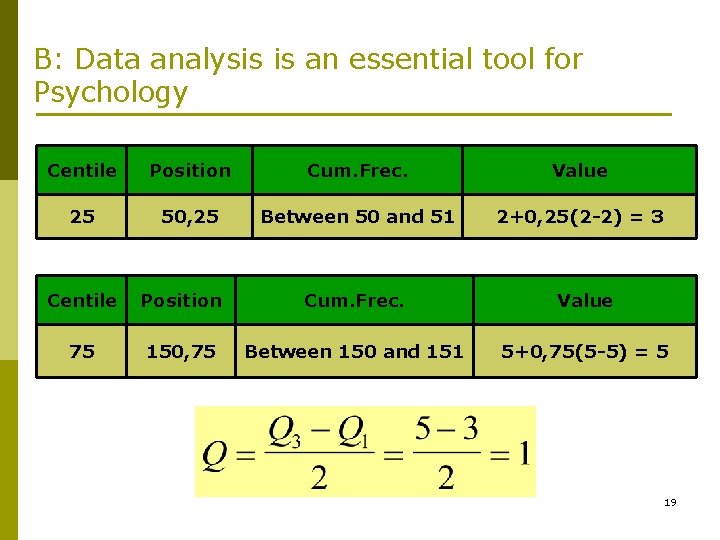
B: Data analysis is an essential tool for Psychology Centile Position Cum. Frec. Value 25 50, 25 Between 50 and 51 2+0, 25(2 -2) = 3 Centile Position Cum. Frec. Value 75 150, 75 Between 150 and 151 5+0, 75(5 -5) = 5 19

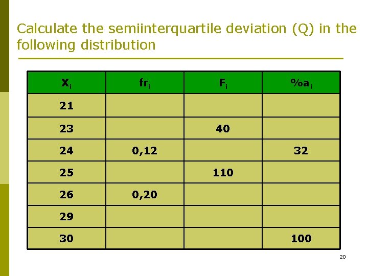
Calculate the semiinterquartile deviation (Q) in the following distribution Xi fri Fi %ai 21 23 24 40 0, 12 25 26 32 110 0, 20 29 30 100 20

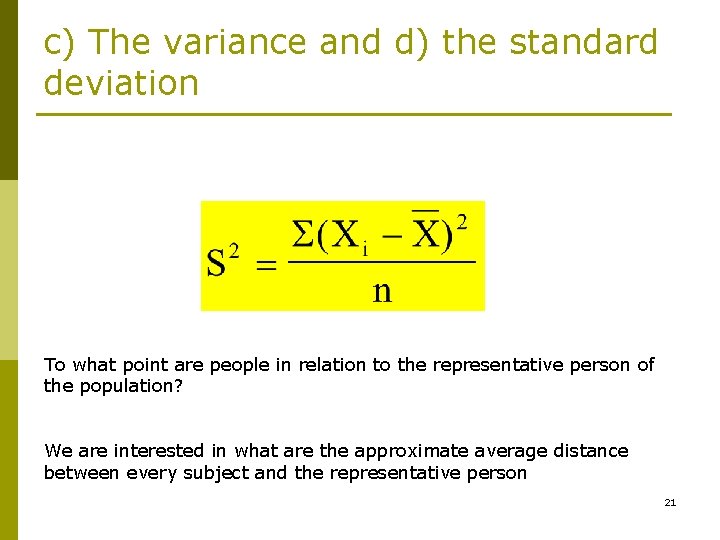
c) The variance and d) the standard deviation To what point are people in relation to the representative person of the population? We are interested in what are the approximate average distance between every subject and the representative person 21

p Same mass above and below the average: to solve this problem we square. p Because of the discrepancies sum, as more data will mean more differences: to avoid this influence of n, divided by n.

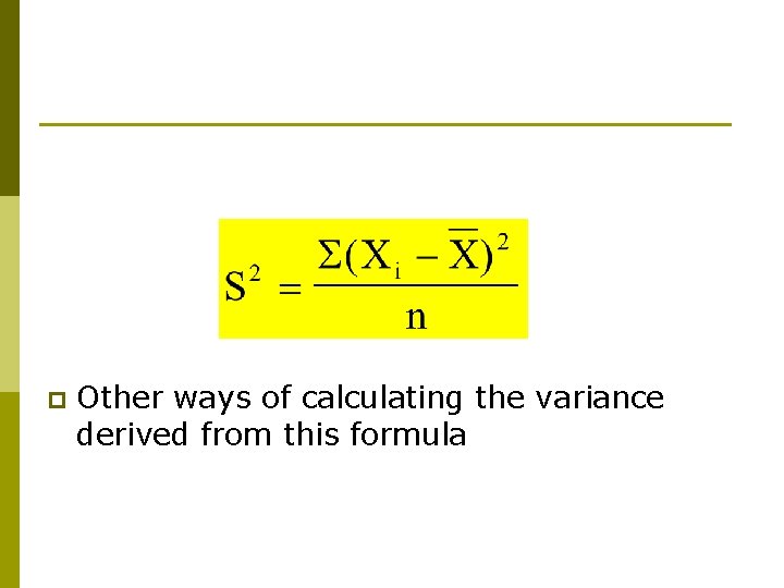
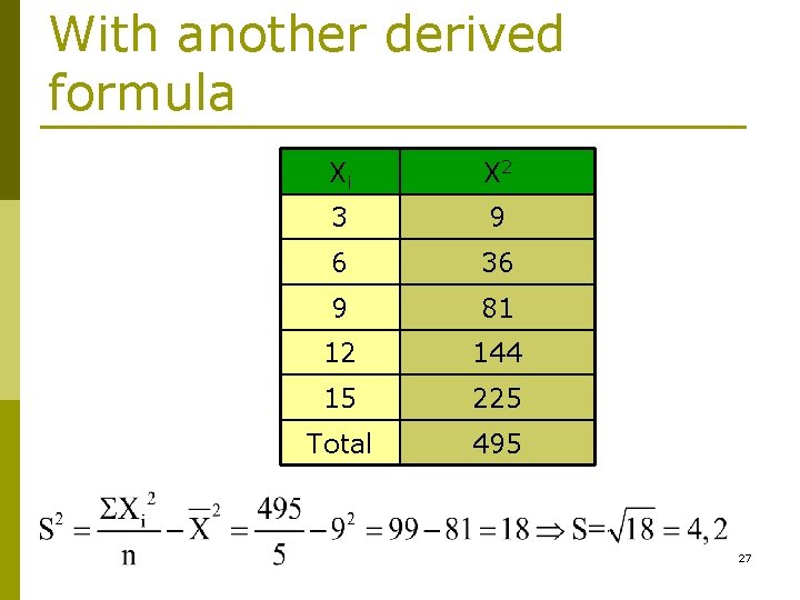
p Other ways of calculating the variance derived from this formula

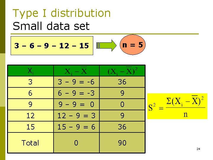
Type I distribution Small data set 3 – 6 – 9 – 12 – 15 n=5 Xi 3 3 – 9 = -6 36 6 6 – 9 = -3 9 9 9– 9= 0 0 12 12 – 9 = 3 9 15 15 – 9 = 6 36 Total 0 90 24

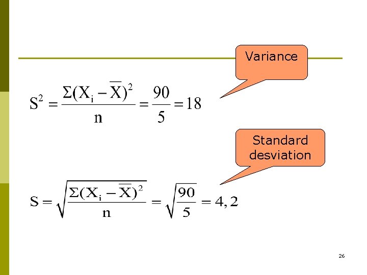
p Variance is expressed in units squared, and this does not usually use. p 2 onions are ok, but 2 onions squared have no sense! p In order to the dispersion is also expressed in the same units as the variable in its origin we do the square root (obtaining the standard deviation).

Variance Standard desviation 26

With another derived formula Xi X 2 3 9 6 36 9 81 12 144 15 225 Total 495 27

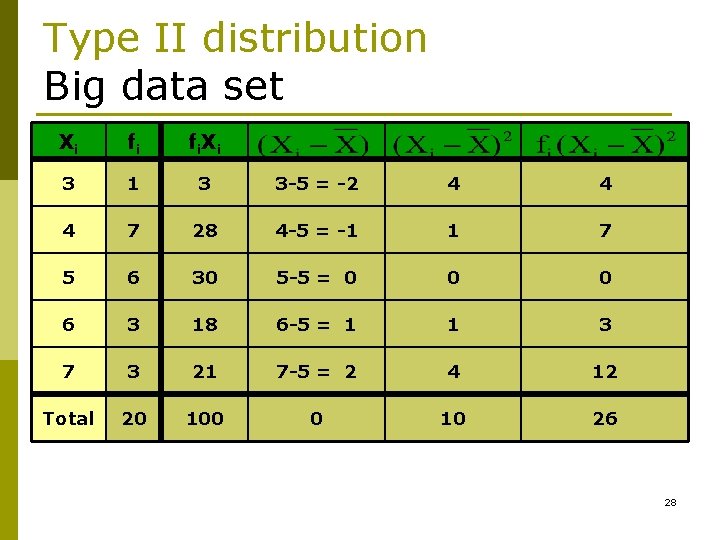
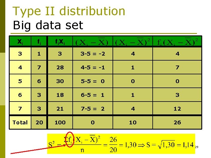
Type II distribution Big data set Xi fi fi. Xi 3 1 3 3 -5 = -2 4 4 4 7 28 4 -5 = -1 1 7 5 6 30 5 -5 = 0 0 0 6 3 18 6 -5 = 1 1 3 7 3 21 7 -5 = 2 4 12 Total 20 100 0 10 26 28

Type II distribution Big data set Xi fi fi. Xi 3 1 3 3 -5 = -2 4 4 4 7 28 4 -5 = -1 1 7 5 6 30 5 -5 = 0 0 0 6 3 18 6 -5 = 1 1 3 7 3 21 7 -5 = 2 4 12 Total 20 100 0 10 26 29

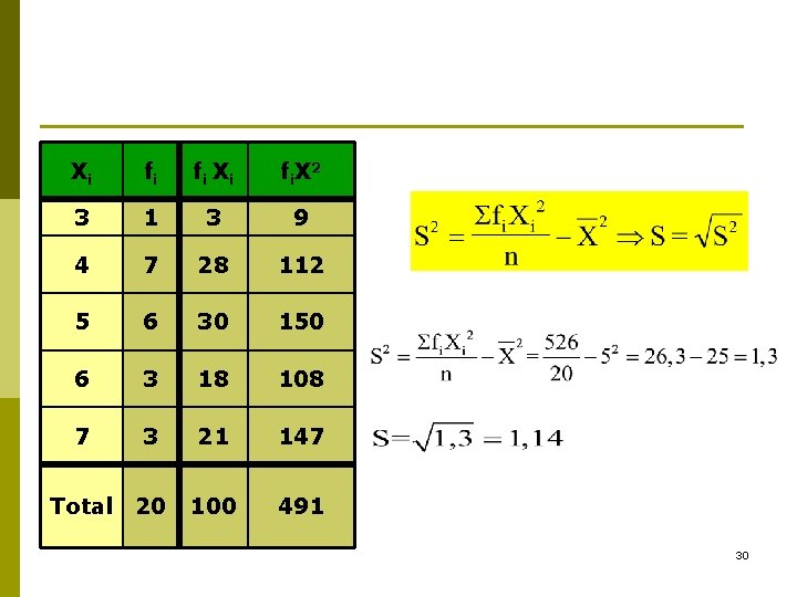
Xi fi fi X i fi. X 2 3 1 3 9 4 7 28 112 5 6 30 150 6 3 18 108 7 3 21 147 100 491 Total 20 30

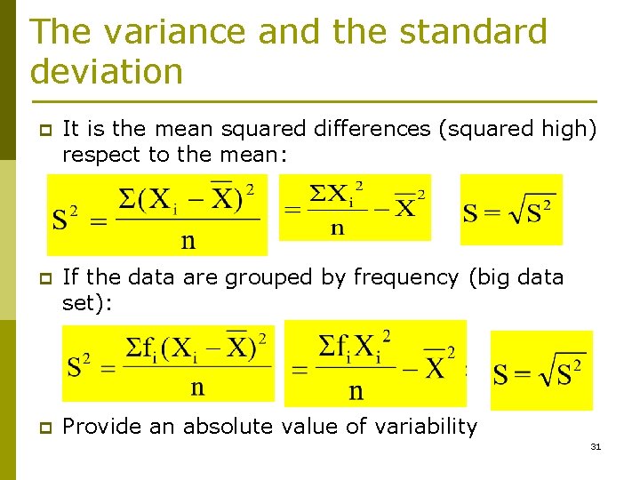
The variance and the standard deviation p It is the mean squared differences (squared high) respect to the mean: p If the data are grouped by frequency (big data set): p Provide an absolute value of variability 31

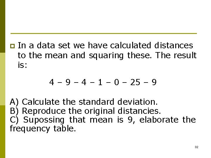
p In a data set we have calculated distances to the mean and squaring these. The result is: 4 – 9 – 4 – 1 – 0 – 25 – 9 A) Calculate the standard deviation. B) Reproduce the original distancies. C) Supossing that mean is 9, elaborate the frequency table. 32

Other dispersion indexes 33

e) The Quasivariance and f) The Standard Quasideviation p It can be used when you want to make a more accurate estimate of the variance and the standard deviation of the population. p When the sample is small, the difference is significant. 34

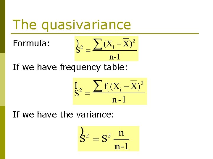
The quasivariance Formula: If we have frequency table: If we have the variance:

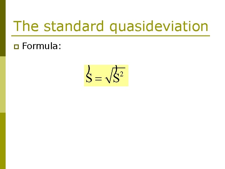
The standard quasideviation p Formula:

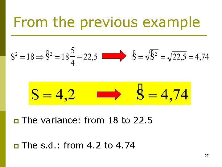
From the previous example p The variance: from 18 to 22. 5 p The s. d. : from 4. 2 to 4. 74 37

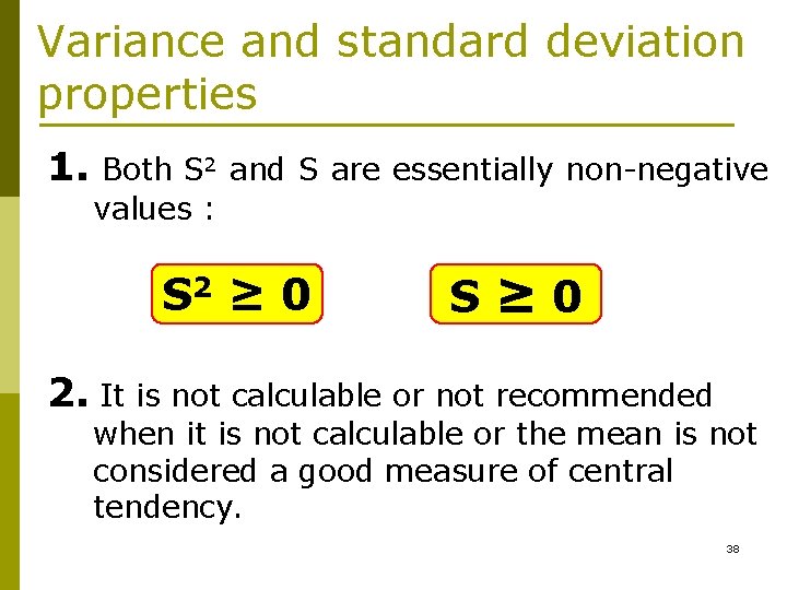
Variance and standard deviation properties 1. Both S 2 and S are essentially non-negative values : S 2 ≥ 0 S≥ 0 2. It is not calculable or not recommended when it is not calculable or the mean is not considered a good measure of central tendency. 38

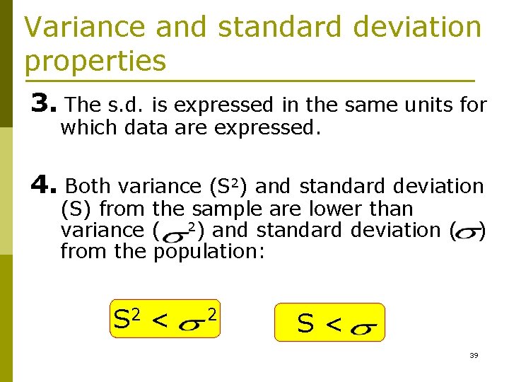
Variance and standard deviation properties 3. The s. d. is expressed in the same units for which data are expressed. 4. Both variance (S 2) and standard deviation (S) from the sample are lower than variance ( 2) and standard deviation ( from the population: S 2 < 2 ) S< 39

g) Pearson’s variation coefficient p Ex: age p A difference of 2 years of age may be a lot or little: n n n p 78 -80 age range 1 -3 age range Does this difference of two years have the same connotations? There is a psychological difference that the numbers can not detect. We, as psychologists (in the near future) have to interpret it. 40

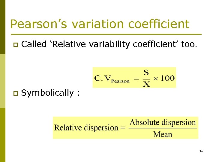
Pearson’s variation coefficient p Called ‘Relative variability coefficient’ too. p Symbolically : 41

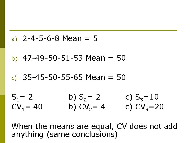
p It is preferable to use the CV before the S when we want to compare the dispersions of two or more distributions of data. p Large units produce larger differences. This is reflected in the mean. p When the means are similar, it is more simple and equally valid comparison in terms of S (calculating the CV does not bring anything new).

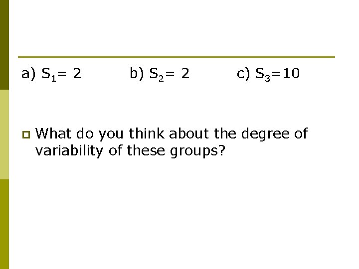
a) S 1= 2 p b) S 2= 2 c) S 3=10 What do you think about the degree of variability of these groups?

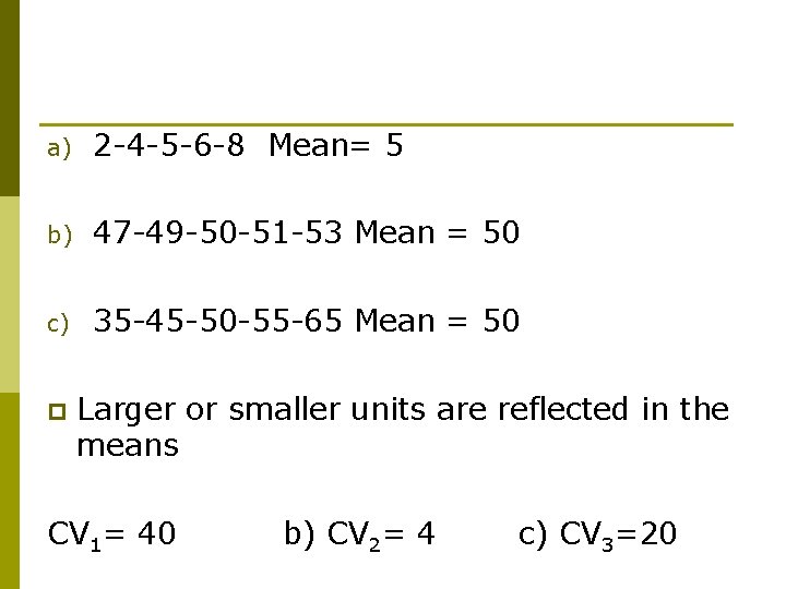
a) 2 -4 -5 -6 -8 Mean= 5 b) 47 -49 -50 -51 -53 Mean = 50 c) 35 -45 -50 -55 -65 Mean = 50 p Larger or smaller units are reflected in the means CV 1= 40 b) CV 2= 4 c) CV 3=20

a) 2 -4 -5 -6 -8 Mean = 5 b) 47 -49 -50 -51 -53 Mean = 50 c) 35 -45 -50 -55 -65 Mean = 50 S 1= 2 CV 1= 40 b) S 2= 2 b) CV 2= 4 c) S 3=10 c) CV 3=20 When the means are equal, CV does not add anything (same conclusions)

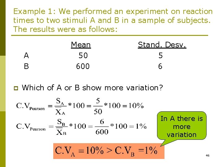
Example 1: We performed an experiment on reaction times to two stimuli A and B in a sample of subjects. The results were as follows: A B p Mean 50 600 Stand. Desv. 5 6 Which of A or B show more variation? In A there is more variation 46

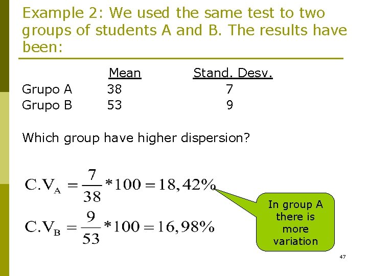
Example 2: We used the same test to two groups of students A and B. The results have been: Grupo A Grupo B Mean 38 53 Stand. Desv. 7 9 Which group have higher dispersion? In group A there is more variation 47

Form measurements 48

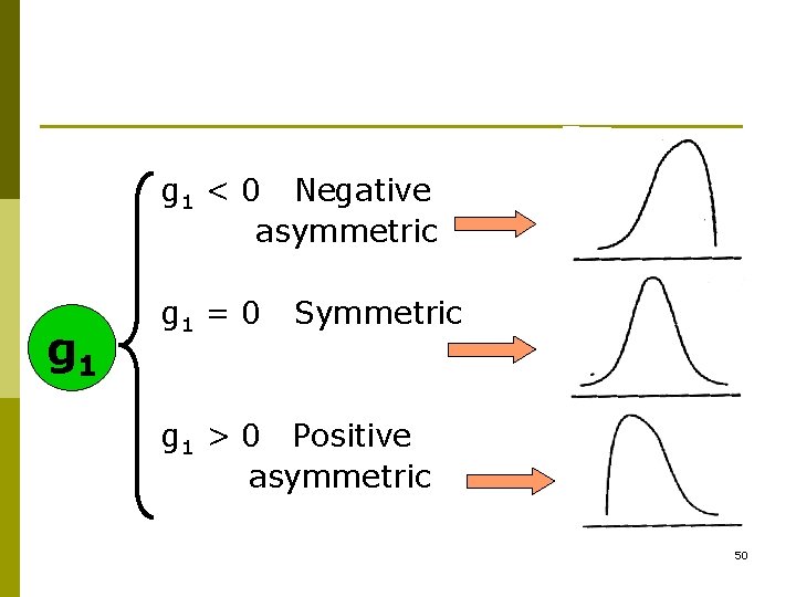
Bias or asimmetry measurements p Two distributions with the same mean and the same dispersion can be, in terms of shape, totally different. p These measures tell us in which distribution side there is a greater dispersion. 49

g 1 < 0 Negative asymmetric g 1 = 0 Symmetric g 1 > 0 Positive asymmetric 50

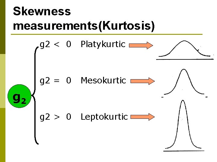
Skewness or Kurtosis measurements p Refers to the distributions degree of pointing or slenderness. p The skewness indicates a marked contrast between the high central frequency and the rest.

Skewness measurements(Kurtosis) g 2 < 0 Platykurtic g 2 = 0 Mesokurtic g 2 > 0 Leptokurtic g 2 52

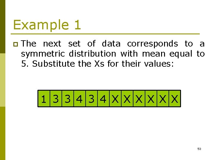
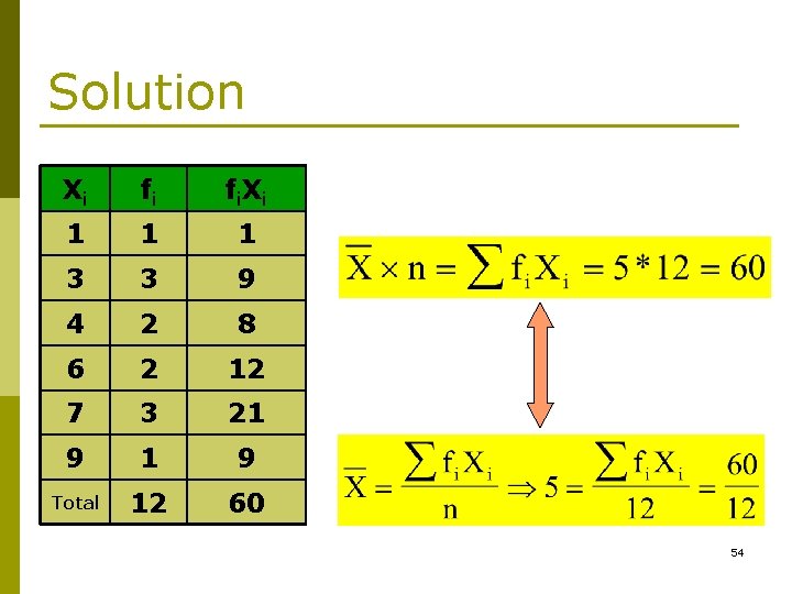
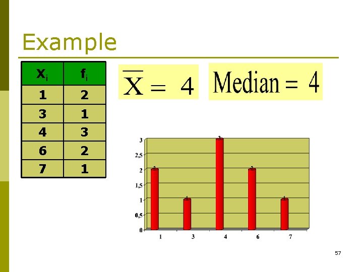
Example 1 p The next set of data corresponds to a symmetric distribution with mean equal to 5. Substitute the Xs for their values: 1 3 3 4 X X X 53

Solution Xi fi fi X i 1 1 1 3 3 9 4 2 8 6 2 12 7 3 21 9 Total 12 60 54

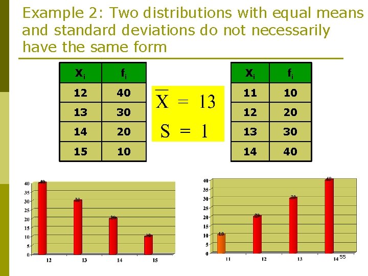
Example 2: Two distributions with equal means and standard deviations do not necessarily have the same form Xi fi 12 40 11 10 13 30 12 20 14 20 13 30 15 10 14 40 55

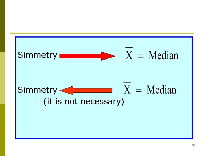
Simmetry (it is not necessary) 56

Example Xi fi 1 2 3 1 4 3 6 2 7 1 57