Chapter 4 EXPONENTIAL FUNCTIONS Section 4 1 Introduction

Chapter 4 EXPONENTIAL FUNCTIONS Section 4. 1 Introduction to the Family of Exponential Functions Section 4. 2 Comparing Exponential and Linear Functions Section 4. 3 Graphs of Exponential Functions Section 4. 4 Applications to Compound Interest Section 4. 5 The Number e Functions Modeling Change: A Preparation for Calculus, 5 th Edition, 2014, Connally 1

4. 1 INTRODUCTION TO THE FAMILY OF EXPONENTIAL FUNCTIONS Functions Modeling Change: A Preparation for Calculus, 5 th Edition, 2014, Connally 2

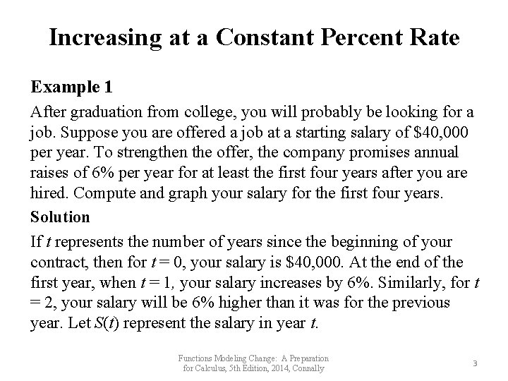
Increasing at a Constant Percent Rate Example 1 After graduation from college, you will probably be looking for a job. Suppose you are offered a job at a starting salary of $40, 000 per year. To strengthen the offer, the company promises annual raises of 6% per year for at least the first four years after you are hired. Compute and graph your salary for the first four years. Solution If t represents the number of years since the beginning of your contract, then for t = 0, your salary is $40, 000. At the end of the first year, when t = 1, your salary increases by 6%. Similarly, for t = 2, your salary will be 6% higher than it was for the previous year. Let S(t) represent the salary in year t. Functions Modeling Change: A Preparation for Calculus, 5 th Edition, 2014, Connally 3

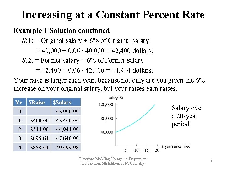
Increasing at a Constant Percent Rate Example 1 Solution continued S(1) = Original salary + 6% of Original salary = 40, 000 + 0. 06 ∙ 40, 000 = 42, 400 dollars. S(2) = Former salary + 6% of Former salary = 42, 400 + 0. 06 ∙ 42, 400 = 44, 944 dollars. Your raise is larger each year, because not only are you given the 6% increase on your original salary, but your raises earn raises. Yr $Raise 0 $Salary over a 20 -year period 42, 000. 00 1 2400. 00 42, 400. 00 2 2544. 00 44, 944. 00 3 2696. 64 47, 640. 00 4 2858. 44 50, 499. 08 Functions Modeling Change: A Preparation for Calculus, 5 th Edition, 2014, Connally 4

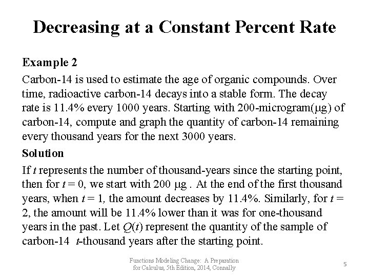
Decreasing at a Constant Percent Rate Example 2 Carbon-14 is used to estimate the age of organic compounds. Over time, radioactive carbon-14 decays into a stable form. The decay rate is 11. 4% every 1000 years. Starting with 200 -microgram( g) of carbon-14, compute and graph the quantity of carbon-14 remaining every thousand years for the next 3000 years. Solution If t represents the number of thousand-years since the starting point, then for t = 0, we start with 200 g. At the end of the first thousand years, when t = 1, the amount decreases by 11. 4%. Similarly, for t = 2, the amount will be 11. 4% lower than it was for one-thousand years in the past. Let Q(t) represent the quantity of the sample of carbon-14 t-thousand years after the starting point. Functions Modeling Change: A Preparation for Calculus, 5 th Edition, 2014, Connally 5

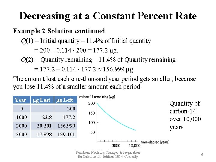
Decreasing at a Constant Percent Rate Example 2 Solution continued Q(1) = Initial quantity – 11. 4% of Initial quantity = 200 – 0. 114 ∙ 200 = 177. 2 g. Q(2) = Quantity remaining – 11. 4% of Quantity remaining = 177. 2 – 0. 114 ∙ 177. 2 ≈ 156. 999 g. The amount lost each one-thousand year period gets smaller, because you lose 11. 4% of a smaller amount each period. Year g Lost 0 g Left Quantity of carbon-14 over 10, 000 years. 200 1000 22. 8 177. 2 2000 20. 201 156. 999 3000 17. 898 139. 101 Functions Modeling Change: A Preparation for Calculus, 5 th Edition, 2014, Connally 6

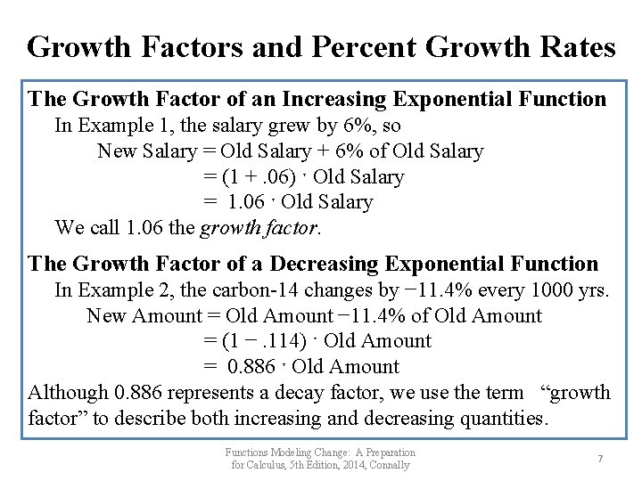
Growth Factors and Percent Growth Rates The Growth Factor of an Increasing Exponential Function In Example 1, the salary grew by 6%, so New Salary = Old Salary + 6% of Old Salary = (1 +. 06) ˑ Old Salary = 1. 06 ˑ Old Salary We call 1. 06 the growth factor. The Growth Factor of a Decreasing Exponential Function In Example 2, the carbon-14 changes by − 11. 4% every 1000 yrs. New Amount = Old Amount − 11. 4% of Old Amount = (1 −. 114) ˑ Old Amount = 0. 886 ˑ Old Amount Although 0. 886 represents a decay factor, we use the term “growth factor” to describe both increasing and decreasing quantities. Functions Modeling Change: A Preparation for Calculus, 5 th Edition, 2014, Connally 7

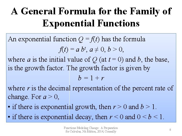
A General Formula for the Family of Exponential Functions An exponential function Q = f(t) has the formula f(t) = a bt, a ≠ 0, b > 0, where a is the initial value of Q (at t = 0) and b, the base, is the growth factor. The growth factor is given by b=1+r where r is the decimal representation of the percent rate of change. For a > 0, • if there is exponential growth, then r > 0 and b > 1. • if there is exponential decay, then r < 0 and 0 < b < 1. Functions Modeling Change: A Preparation for Calculus, 5 th Edition, 2014, Connally 8

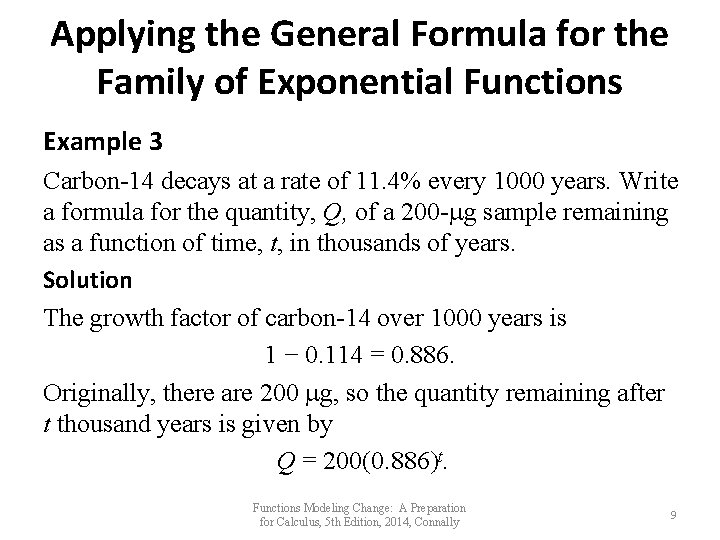
Applying the General Formula for the Family of Exponential Functions Example 3 Carbon-14 decays at a rate of 11. 4% every 1000 years. Write a formula for the quantity, Q, of a 200 - g sample remaining as a function of time, t, in thousands of years. Solution The growth factor of carbon-14 over 1000 years is 1 − 0. 114 = 0. 886. Originally, there are 200 g, so the quantity remaining after t thousand years is given by Q = 200(0. 886)t. Functions Modeling Change: A Preparation for Calculus, 5 th Edition, 2014, Connally 9

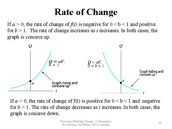
Rate of Change If a > 0, the rate of change of f(t) is negative for 0 < b < 1 and positive for b > 1. The rate of change increases as t increases. In both cases, the graph is concave up. If a < 0, the rate of change of f(t) is positive for 0 < b < 1 and negative for b > 1. The rate of change decreases as t increases. In both cases, the graph is concave down. Functions Modeling Change: A Preparation for Calculus, 5 th Edition, 2014, Connally 10

4. 2 COMPARING EXPONENTIAL AND LINEAR FUNCTIONS Functions Modeling Change: A Preparation for Calculus, 5 th Edition, 2014, Connally 11

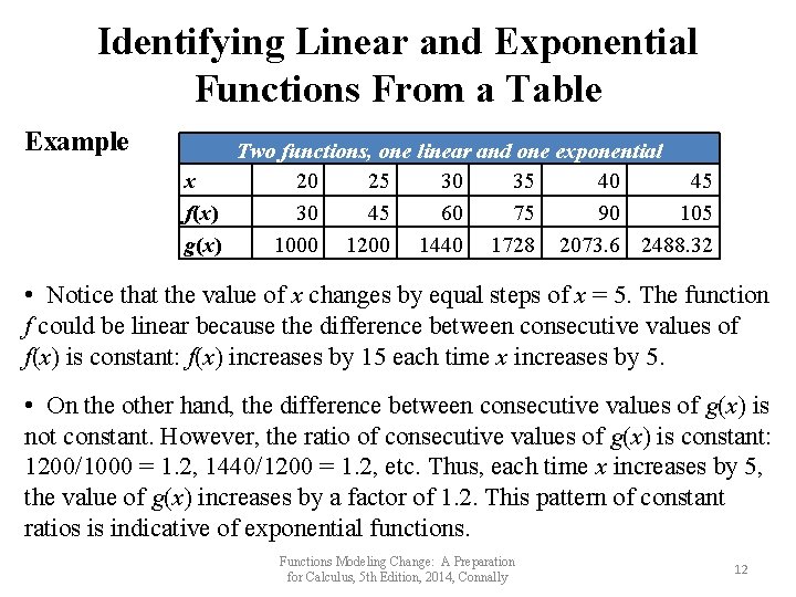
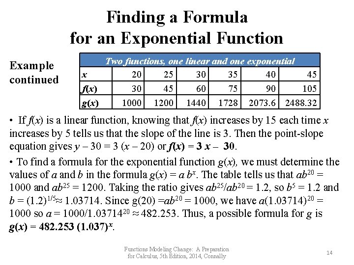
Identifying Linear and Exponential Functions From a Table Example Two functions, one linear and one exponential x 20 25 30 35 40 45 f(x) 30 45 60 75 90 105 g(x) 1000 1200 1440 1728 2073. 6 2488. 32 • Notice that the value of x changes by equal steps of x = 5. The function f could be linear because the difference between consecutive values of f(x) is constant: f(x) increases by 15 each time x increases by 5. • On the other hand, the difference between consecutive values of g(x) is not constant. However, the ratio of consecutive values of g(x) is constant: 1200/1000 = 1. 2, 1440/1200 = 1. 2, etc. Thus, each time x increases by 5, the value of g(x) increases by a factor of 1. 2. This pattern of constant ratios is indicative of exponential functions. Functions Modeling Change: A Preparation for Calculus, 5 th Edition, 2014, Connally 12

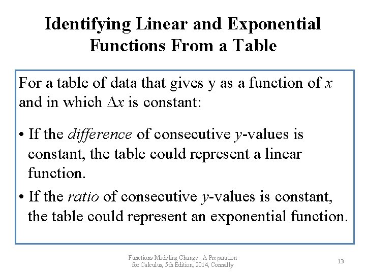
Identifying Linear and Exponential Functions From a Table For a table of data that gives y as a function of x and in which x is constant: • If the difference of consecutive y-values is constant, the table could represent a linear function. • If the ratio of consecutive y-values is constant, the table could represent an exponential function. Functions Modeling Change: A Preparation for Calculus, 5 th Edition, 2014, Connally 13

Finding a Formula for an Exponential Function Example continued Two functions, one linear and one exponential x 20 25 30 35 40 45 f(x) 30 45 60 75 90 105 g(x) 1000 1200 1440 1728 2073. 6 2488. 32 • If f(x) is a linear function, knowing that f(x) increases by 15 each time x increases by 5 tells us that the slope of the line is 3. Then the point-slope equation gives y – 30 = 3 (x – 20) or f(x) = 3 x – 30. • To find a formula for the exponential function g(x), we must determine the values of a and b in the formula g(x) = a bx. The table tells us that ab 20 = 1000 and ab 25 = 1200. Taking the ratio gives ab 25/ab 20 = 1. 2, so b 5 = 1. 2 and b = (1. 2)1/5≈ 1. 03714. Since g(20) =ab 20 = 1000, we have a(1. 03714)20 = 1000 so a = 1000/1. 0371420 ≈ 482. 253. Thus, a possible formula for g is g(x) = 482. 253 (1. 037)x. Functions Modeling Change: A Preparation for Calculus, 5 th Edition, 2014, Connally 14

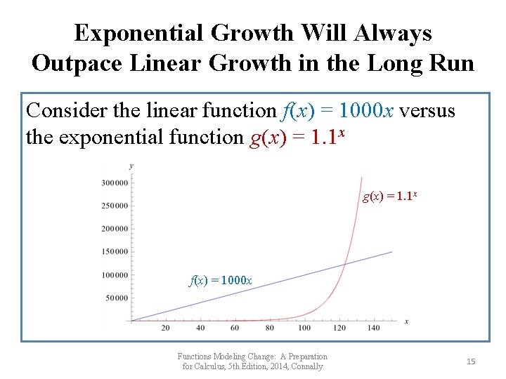
Exponential Growth Will Always Outpace Linear Growth in the Long Run Consider the linear function f(x) = 1000 x versus the exponential function g(x) = 1. 1 x f(x) = 1000 x Functions Modeling Change: A Preparation for Calculus, 5 th Edition, 2014, Connally 15

4. 3 GRAPHS OF EXPONENTIAL FUNCTIONS Functions Modeling Change: A Preparation for Calculus, 5 th Edition, 2014, Connally 16

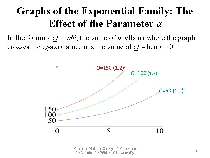
Graphs of the Exponential Family: The Effect of the Parameter a In the formula Q = abt, the value of a tells us where the graph crosses the Q-axis, since a is the value of Q when t = 0. Q=150 (1. 2)t Q=100 (1. 2)t Q=50 (1. 2)t Functions Modeling Change: A Preparation for Calculus, 5 th Edition, 2014, Connally 17

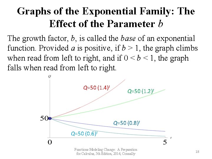
Graphs of the Exponential Family: The Effect of the Parameter b The growth factor, b, is called the base of an exponential function. Provided a is positive, if b > 1, the graph climbs when read from left to right, and if 0 < b < 1, the graph falls when read from left to right. Q=50 (1. 4)t Q=50 (1. 2)t Q=50 (0. 8)t Q=50 (0. 6)t Functions Modeling Change: A Preparation for Calculus, 5 th Edition, 2014, Connally 18

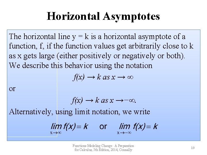
Horizontal Asymptotes The horizontal line y = k is a horizontal asymptote of a function, f, if the function values get arbitrarily close to k as x gets large (either positively or negatively or both). We describe this behavior using the notation f(x) → k as x → ∞ or f(x) → k as x →−∞. Alternatively, using limit notation, we write Functions Modeling Change: A Preparation for Calculus, 5 th Edition, 2014, Connally 19

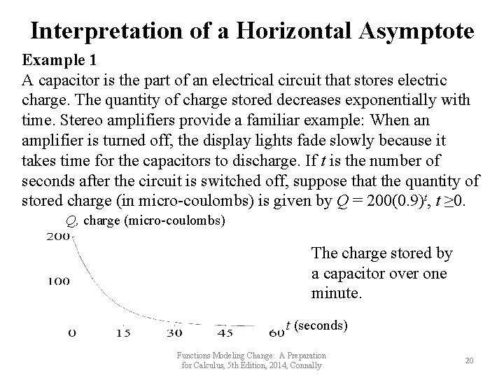
Interpretation of a Horizontal Asymptote Example 1 A capacitor is the part of an electrical circuit that stores electric charge. The quantity of charge stored decreases exponentially with time. Stereo amplifiers provide a familiar example: When an amplifier is turned off, the display lights fade slowly because it takes time for the capacitors to discharge. If t is the number of seconds after the circuit is switched off, suppose that the quantity of stored charge (in micro-coulombs) is given by Q = 200(0. 9)t, t ≥ 0. Q, charge (micro-coulombs) The charge stored by a capacitor over one minute. t (seconds) Functions Modeling Change: A Preparation for Calculus, 5 th Edition, 2014, Connally 20

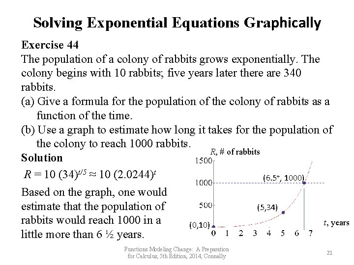
Solving Exponential Equations Graphically Exercise 44 The population of a colony of rabbits grows exponentially. The colony begins with 10 rabbits; five years later there are 340 rabbits. (a) Give a formula for the population of the colony of rabbits as a function of the time. (b) Use a graph to estimate how long it takes for the population of the colony to reach 1000 rabbits. R, # of rabbits Solution R = 10 (34)t/5 ≈ 10 (2. 0244)t (6. 5+, 1000) Based on the graph, one would estimate that the population of (5, 34) rabbits would reach 1000 in a t, years (0, 10) little more than 6 ½ years. Functions Modeling Change: A Preparation for Calculus, 5 th Edition, 2014, Connally 21

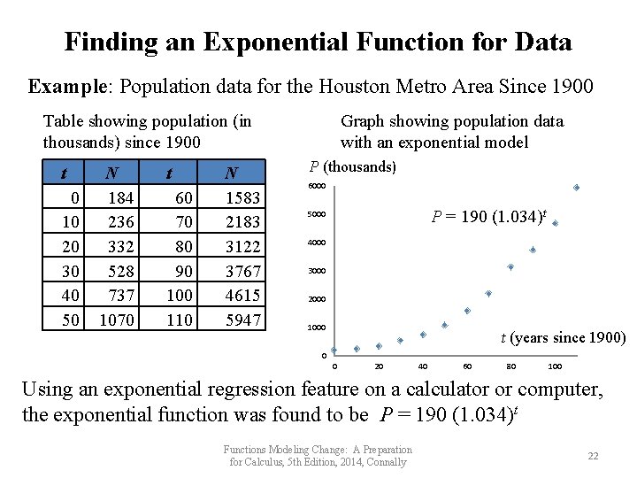
Finding an Exponential Function for Data Example: Population data for the Houston Metro Area Since 1900 Table showing population (in thousands) since 1900 t 0 10 20 30 40 50 N 184 236 332 528 737 1070 t 60 70 80 90 100 110 N 1583 2183 3122 3767 4615 5947 Graph showing population data with an exponential model P (thousands) 6000 P = 190 (1. 034)t 5000 4000 3000 2000 1000 t (years since 1900) 0 0 20 40 60 80 100 Using an exponential regression feature on a calculator or computer, the exponential function was found to be P = 190 (1. 034)t Functions Modeling Change: A Preparation for Calculus, 5 th Edition, 2014, Connally 22

4. 4 APPLICATIONS TO COMPOUND INTEREST Functions Modeling Change: A Preparation for Calculus, 5 th Edition, 2014, Connally 23

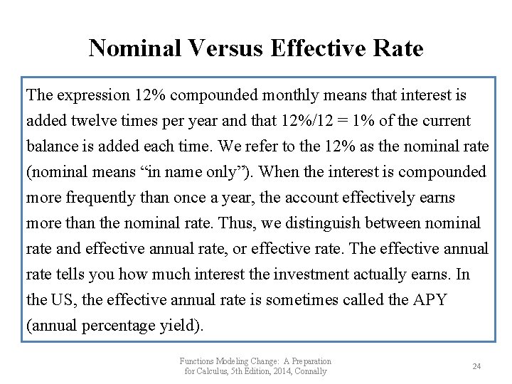
Nominal Versus Effective Rate The expression 12% compounded monthly means that interest is added twelve times per year and that 12%/12 = 1% of the current balance is added each time. We refer to the 12% as the nominal rate (nominal means “in name only”). When the interest is compounded more frequently than once a year, the account effectively earns more than the nominal rate. Thus, we distinguish between nominal rate and effective annual rate, or effective rate. The effective annual rate tells you how much interest the investment actually earns. In the US, the effective annual rate is sometimes called the APY (annual percentage yield). Functions Modeling Change: A Preparation for Calculus, 5 th Edition, 2014, Connally 24

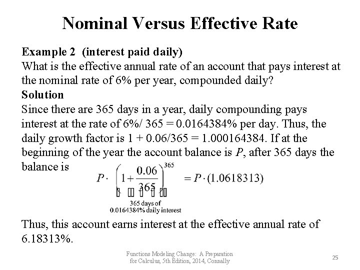
Nominal Versus Effective Rate Example 2 (interest paid daily) What is the effective annual rate of an account that pays interest at the nominal rate of 6% per year, compounded daily? Solution Since there are 365 days in a year, daily compounding pays interest at the rate of 6%/ 365 = 0. 0164384% per day. Thus, the daily growth factor is 1 + 0. 06/365 = 1. 000164384. If at the beginning of the year the account balance is P, after 365 days the balance is Thus, this account earns interest at the effective annual rate of 6. 18313%. Functions Modeling Change: A Preparation for Calculus, 5 th Edition, 2014, Connally 25

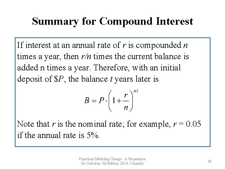
Summary for Compound Interest If interest at an annual rate of r is compounded n times a year, then r/n times the current balance is added n times a year. Therefore, with an initial deposit of $P, the balance t years later is Note that r is the nominal rate; for example, r = 0. 05 if the annual rate is 5%. Functions Modeling Change: A Preparation for Calculus, 5 th Edition, 2014, Connally 26

4. 5 THE NUMBER e Functions Modeling Change: A Preparation for Calculus, 5 th Edition, 2014, Connally 27

The Natural Number e An irrational number, introduced by Euler in 1727, is so important that it is given a special name, e. Its value is approximately e ≈ 2. 71828. . It is often used for the base, b, of the exponential function. Base e is called the natural base. This may seem mysterious, as what could possibly be natural about using an irrational base such as e? The answer is that the formulas of calculus are much simpler if e is used as the base for exponentials. Functions Modeling Change: A Preparation for Calculus, 5 th Edition, 2014, Connally 28

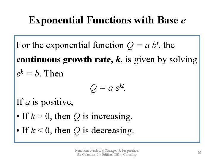
Exponential Functions with Base e For the exponential function Q = a bt, the continuous growth rate, k, is given by solving ek = b. Then Q = a ekt. If a is positive, • If k > 0, then Q is increasing. • If k < 0, then Q is decreasing. Functions Modeling Change: A Preparation for Calculus, 5 th Edition, 2014, Connally 29

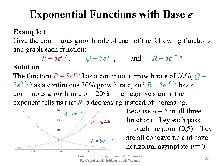
Exponential Functions with Base e Example 1 Give the continuous growth rate of each of the following functions and graph each function: P = 5 e 0. 2 t, Q = 5 e 0. 3 t, and R = 5 e− 0. 2 t. Solution The function P = 5 e 0. 2 t has a continuous growth rate of 20%, Q = 5 e 0. 3 t has a continuous 30% growth rate, and R = 5 e− 0. 2 t has a continuous growth rate of − 20%. The negative sign in the exponent tells us that R is decreasing instead of increasing. Because a = 5 in all three Q = 5 e 0. 3 t functions, they each pass P = 5 e 0. 2 t through the point (0, 5). They are all concave up and have R = 5 e− 0. 2 t horizontal asymptote y = 0. Functions Modeling Change: A Preparation for Calculus, 5 th Edition, 2014, Connally 30

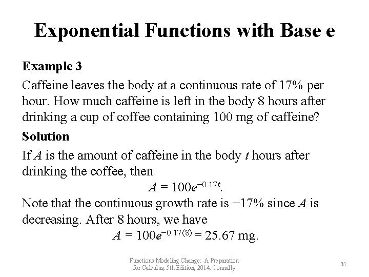
Exponential Functions with Base e Example 3 Caffeine leaves the body at a continuous rate of 17% per hour. How much caffeine is left in the body 8 hours after drinking a cup of coffee containing 100 mg of caffeine? Solution If A is the amount of caffeine in the body t hours after drinking the coffee, then A = 100 e− 0. 17 t. Note that the continuous growth rate is − 17% since A is decreasing. After 8 hours, we have A = 100 e− 0. 17(8) = 25. 67 mg. Functions Modeling Change: A Preparation for Calculus, 5 th Edition, 2014, Connally 31

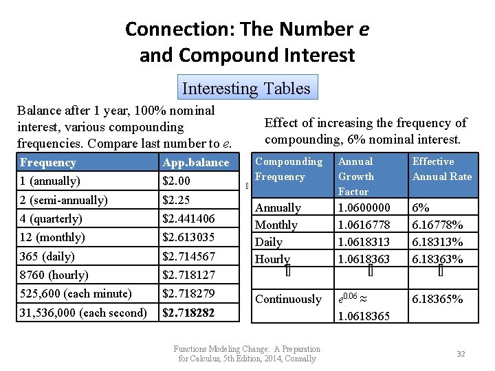
Connection: The Number e and Compound Interesting Tables Balance after 1 year, 100% nominal interest, various compounding frequencies. Compare last number to e. Frequency App. balance 1 (annually) $2. 00 2 (semi-annually) $2. 25 4 (quarterly) $2. 441406 12 (monthly) $2. 613035 365 (daily) $2. 714567 8760 (hourly) $2. 718127 525, 600 (each minute) $2. 718279 31, 536, 000 (each second) $2. 718282 Effect of increasing the frequency of compounding, 6% nominal interest. Compounding Frequency Annual Growth Factor Effective Annual Rate Annually Monthly Daily Hourly 1. 0600000 1. 0616778 1. 0618313 1. 0618363 6% 6. 16778% 6. 18313% 6. 18363% Continuously e 0. 06 ≈ 1. 0618365 6. 18365% Functions Modeling Change: A Preparation for Calculus, 5 th Edition, 2014, Connally 32

Connection: The Number e and Compound Interest If interest on an initial deposit of $P is compounded continuously at a nominal rate of r per year, the balance t years later can be calculated using the formula B = P ert. For example, if the nominal rate is 6%, then r = 0. 06. Functions Modeling Change: A Preparation for Calculus, 5 th Edition, 2014, Connally 33

Exponential Functions with Base e Example 4 An investment has a yield equivalent to a 2. 323% continuous yearly rate. Find the effective annual rate. Solution Since e 0. 02323 = 1. 0235, the effective annual rate is 2. 35%. As expected, the effective annual rate is larger than the continuous yearly rate. Functions Modeling Change: A Preparation for Calculus, 5 th Edition, 2014, Connally 34