Chapter 4 Excel Summarising bivariate data Correlation coefficient

Chapter 4 Excel: Summarising bivariate data

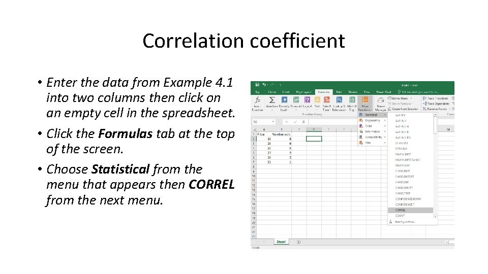
Correlation coefficient • Enter the data from Example 4. 1 into two columns then click on an empty cell in the spreadsheet. • Click the Formulas tab at the top of the screen. • Choose Statistical from the menu that appears then CORREL from the next menu.

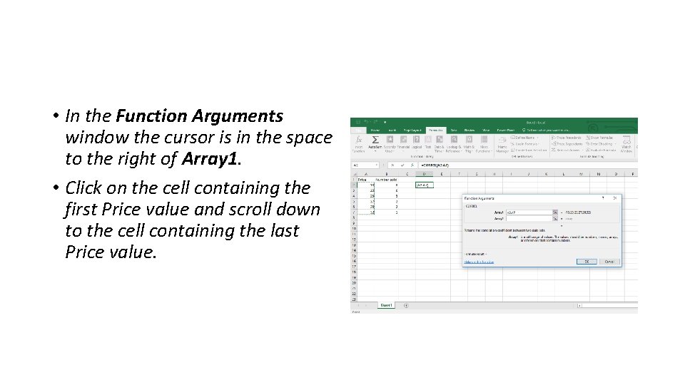
• In the Function Arguments window the cursor is in the space to the right of Array 1. • Click on the cell containing the first Price value and scroll down to the cell containing the last Price value.

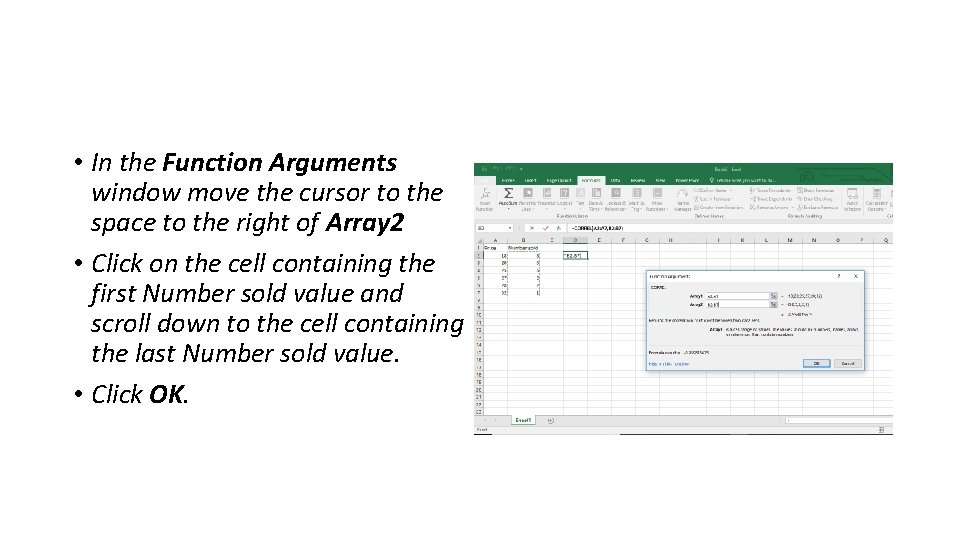
• In the Function Arguments window move the cursor to the space to the right of Array 2 • Click on the cell containing the first Number sold value and scroll down to the cell containing the last Number sold value. • Click OK.

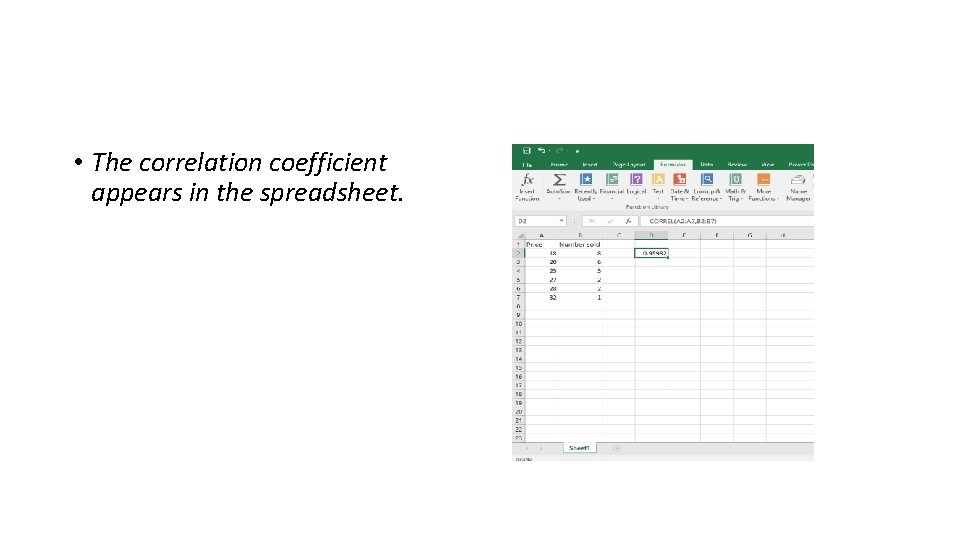
• The correlation coefficient appears in the spreadsheet.

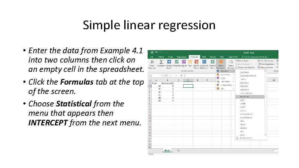
Simple linear regression • Enter the data from Example 4. 1 into two columns then click on an empty cell in the spreadsheet. • Click the Formulas tab at the top of the screen. • Choose Statistical from the menu that appears then INTERCEPT from the next menu.

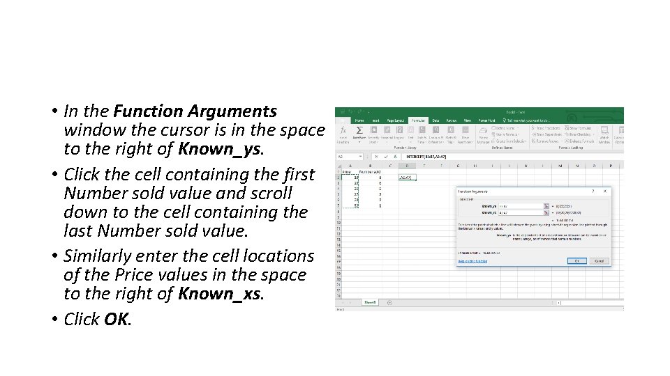
• In the Function Arguments window the cursor is in the space to the right of Known_ys. • Click the cell containing the first Number sold value and scroll down to the cell containing the last Number sold value. • Similarly enter the cell locations of the Price values in the space to the right of Known_xs. • Click OK.

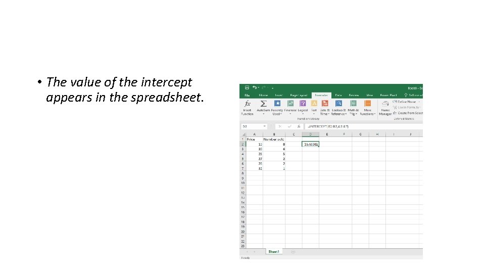
• The value of the intercept appears in the spreadsheet.

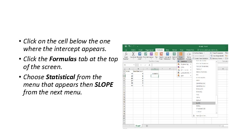
• Click on the cell below the one where the intercept appears. • Click the Formulas tab at the top of the screen. • Choose Statistical from the menu that appears then SLOPE from the next menu.

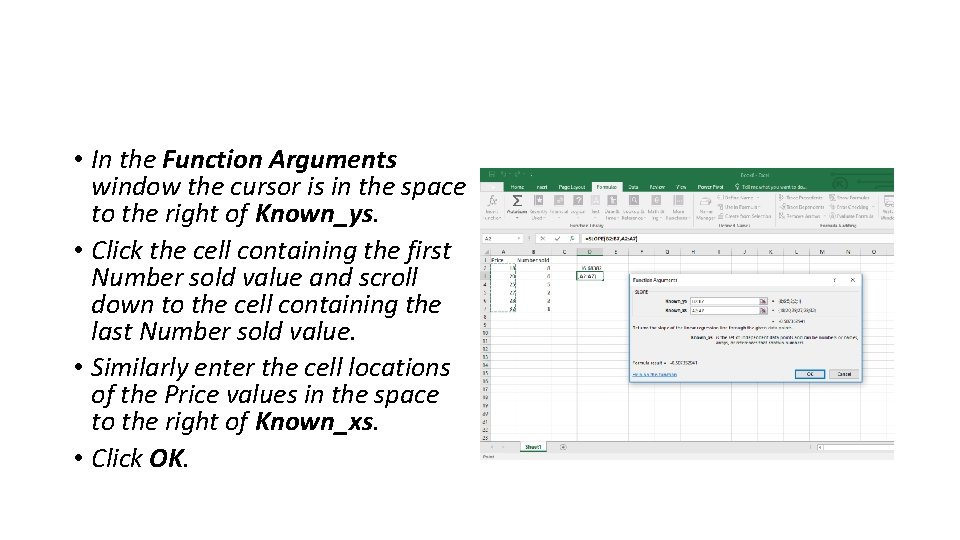
• In the Function Arguments window the cursor is in the space to the right of Known_ys. • Click the cell containing the first Number sold value and scroll down to the cell containing the last Number sold value. • Similarly enter the cell locations of the Price values in the space to the right of Known_xs. • Click OK.

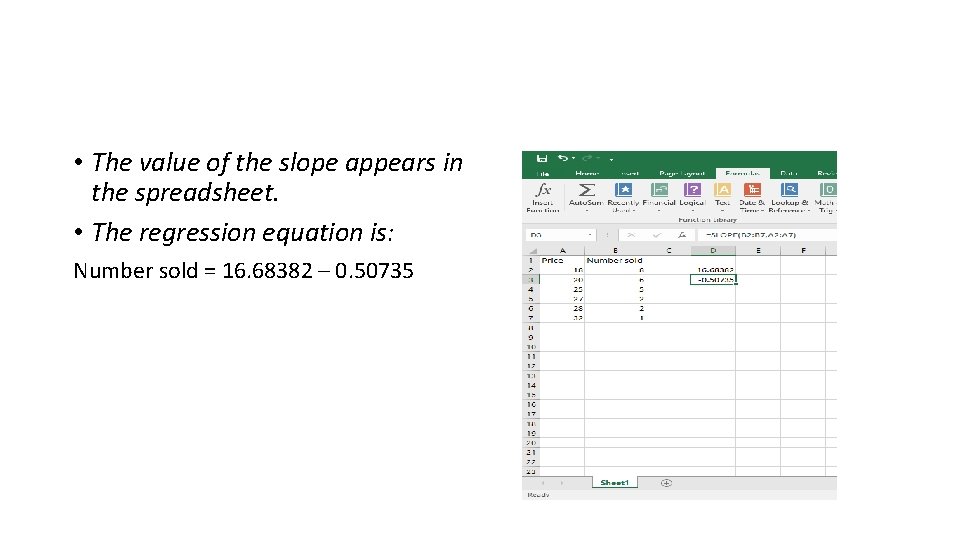
• The value of the slope appears in the spreadsheet. • The regression equation is: Number sold = 16. 68382 – 0. 50735

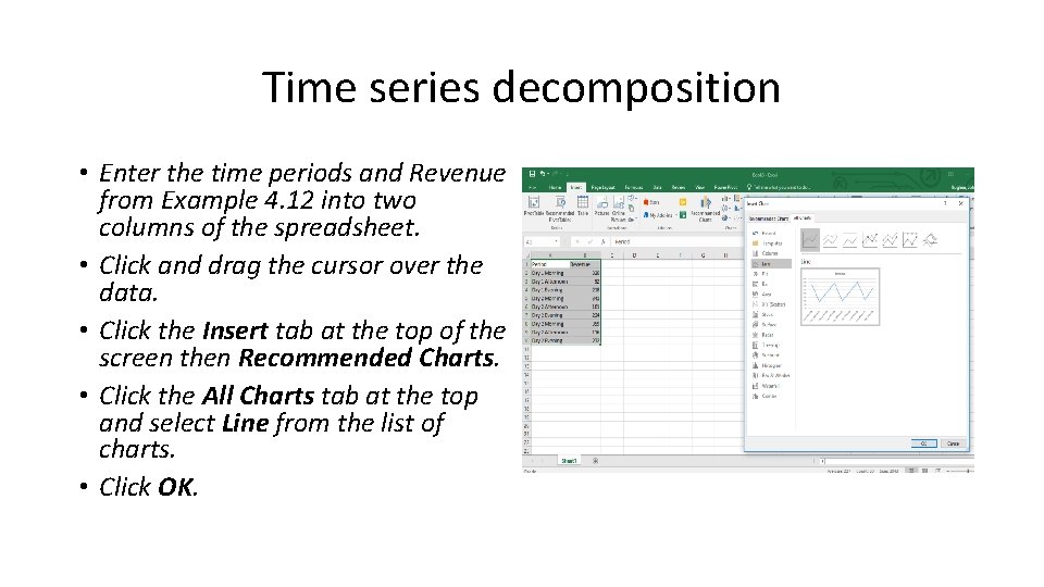
Time series decomposition • Enter the time periods and Revenue from Example 4. 12 into two columns of the spreadsheet. • Click and drag the cursor over the data. • Click the Insert tab at the top of the screen then Recommended Charts. • Click the All Charts tab at the top and select Line from the list of charts. • Click OK.

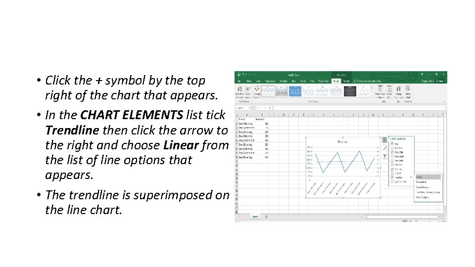
• Click the + symbol by the top right of the chart that appears. • In the CHART ELEMENTS list tick Trendline then click the arrow to the right and choose Linear from the list of line options that appears. • The trendline is superimposed on the line chart.