Chapter 4 Excel Extension Now You Try Using

Chapter 4 Excel Extension: Now You Try! Using the Chi-Square Test to Assess Disparate Impact Bauer, Human Resource Management, First Edition. SAGE Publishing, 2020.

Background In this Excel Extension tutorial, you will learn how to apply the chi-square test of independence to assess disparate impact using Microsoft Excel. For the purposes of this exercise, imagine that you have already queried the frequencies/counts of men and women who passed or failed a knowledge test as well as the frequencies/counts of men and women who passed or failed a physical ability test used for selection. As such, with the observed data in hand, now you’re ready to apply the chi-square test of independence to assess whethere is prima facie evidence of disparate impact, which is sometimes referred to as adverse impact. Bauer, Human Resource Management, First Edition. SAGE Publishing, 2020.

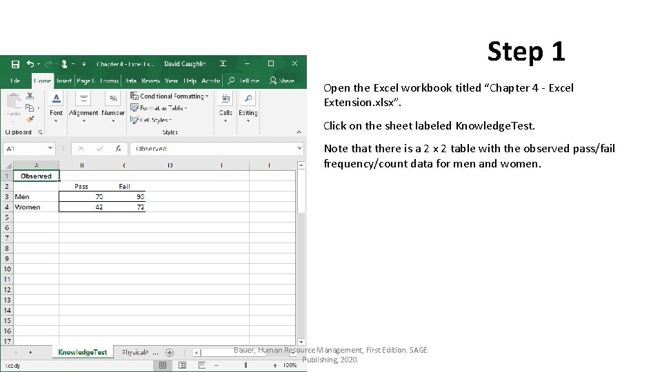
Step 1 Open the Excel workbook titled “Chapter 4 - Excel Extension. xlsx”. Click on the sheet labeled Knowledge. Test. Note that there is a 2 x 2 table with the observed pass/fail frequency/count data for men and women. Bauer, Human Resource Management, First Edition. SAGE Publishing, 2020.

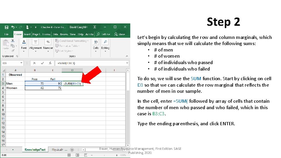
Step 2 Let’s begin by calculating the row and column marginals, which simply means that we will calculate the following sums: • # of men • # of women • # of individuals who passed • # of individuals who failed To do so, we will use the SUM function. Start by clicking on cell D 3 so that we can calculate the row marginal that reflects the number of men in our sample. In the cell, enter =SUM( followed by array of cells that contain the number of men who passed and who failed, which in this case is B 3: C 3. Type the ending parenthesis, and click ENTER. Bauer, Human Resource Management, First Edition. SAGE Publishing, 2020.

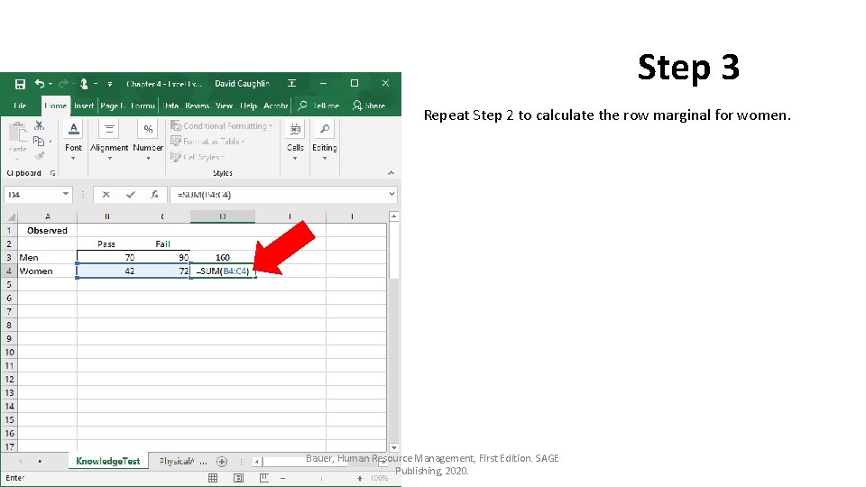
Step 3 Repeat Step 2 to calculate the row marginal for women. Bauer, Human Resource Management, First Edition. SAGE Publishing, 2020.

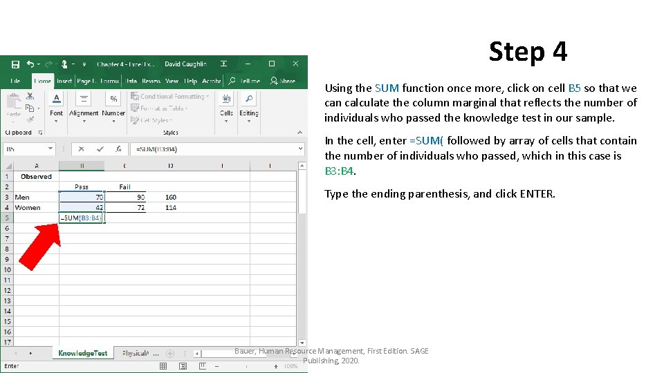
Step 4 Using the SUM function once more, click on cell B 5 so that we can calculate the column marginal that reflects the number of individuals who passed the knowledge test in our sample. In the cell, enter =SUM( followed by array of cells that contain the number of individuals who passed, which in this case is B 3: B 4. Type the ending parenthesis, and click ENTER. Bauer, Human Resource Management, First Edition. SAGE Publishing, 2020.

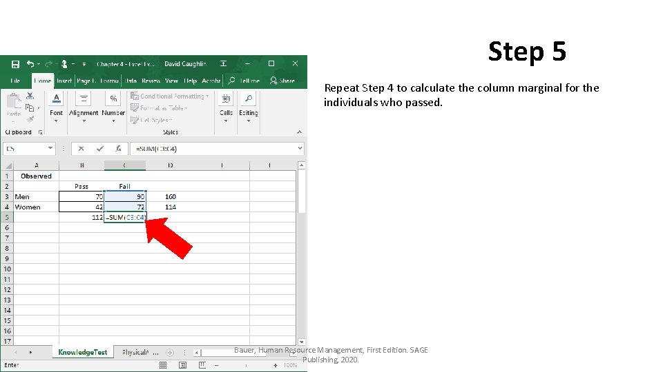
Step 5 Repeat Step 4 to calculate the column marginal for the individuals who passed. Bauer, Human Resource Management, First Edition. SAGE Publishing, 2020.

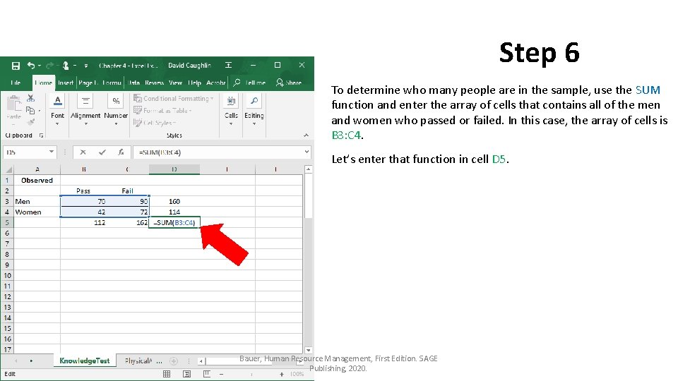
Step 6 To determine who many people are in the sample, use the SUM function and enter the array of cells that contains all of the men and women who passed or failed. In this case, the array of cells is B 3: C 4. Let’s enter that function in cell D 5. Bauer, Human Resource Management, First Edition. SAGE Publishing, 2020.

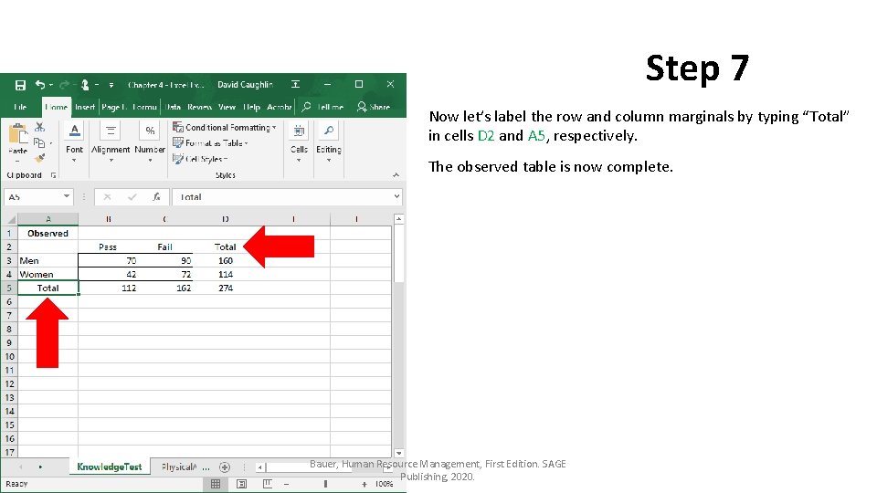
Step 7 Now let’s label the row and column marginals by typing “Total” in cells D 2 and A 5, respectively. The observed table is now complete. Bauer, Human Resource Management, First Edition. SAGE Publishing, 2020.

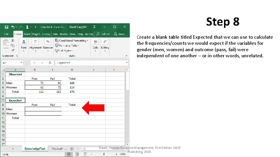
Step 8 Create a blank table titled Expected that we can use to calculate the frequencies/counts we would expect if the variables for gender (men, women) and outcome (pass, fail) were independent of one another – or in other words, unrelated. Bauer, Human Resource Management, First Edition. SAGE Publishing, 2020.

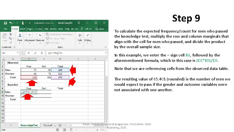
Step 9 To calculate the expected frequency/count for men who passed the knowledge test, multiply the row and column marginals that align with the cell for men who passed, and divide the product by the overall sample size. In this example, we enter the = sign cell B 9, followed by the aforementioned formula, which in this case is (D 3*B 5)/D 5. Note that we are referencing cells from the observed data table. The resulting value of 65. 401 (rounded) is the number of men we would expect to pass if the gender and outcome variables were not associated with one another. Bauer, Human Resource Management, First Edition. SAGE Publishing, 2020.

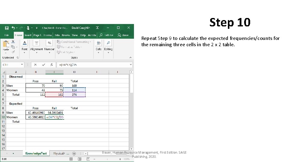
Step 10 Repeat Step 9 to calculate the expected frequencies/counts for the remaining three cells in the 2 x 2 table. Bauer, Human Resource Management, First Edition. SAGE Publishing, 2020.

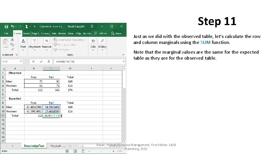
Step 11 Just as we did with the observed table, let’s calculate the row and column marginals using the SUM function. Note that the marginal values are the same for the expected table as they are for the observed table. Bauer, Human Resource Management, First Edition. SAGE Publishing, 2020.

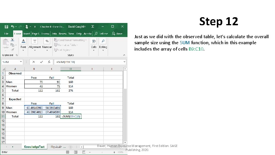
Step 12 Just as we did with the observed table, let’s calculate the overall sample size using the SUM function, which in this example includes the array of cells B 9: C 10. Bauer, Human Resource Management, First Edition. SAGE Publishing, 2020.

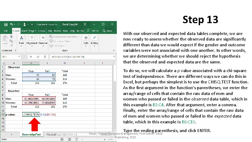
Step 13 With our observed and expected data tables complete, we are now ready to assess whether the observed data are significantly different than data we would expect if the gender and outcome variables were not associated with one another. In other words, we are determining whether we should reject the hypothesis that the observed and expected data are the same. To do so, we will calculate a p value associated with a chi-square test of independence. There are different ways we can do this in Excel, but perhaps the simplest is to use the CHISQ. TEST function. As the first argument in the function’s parentheses, we enter the array/range of cells that contain the raw data of men and women who passed or failed in the observed data table, which in this example is B 3: C 4. After that argument, enter a comma. Finally, enter the array/range of cells that contain the raw data of men and women who passed or failed in the expected data table, which in this example is B 9: C 10. Type the ending parenthesis, and click ENTER. Bauer, Human Resource Management, First Edition. SAGE Publishing, 2020.

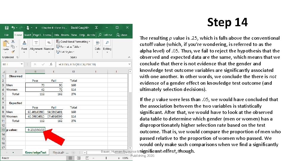
Step 14 The resulting p value is. 25, which is falls above the conventional cutoff value (which, if you’re wondering, is referred to as the alpha level) of. 05. Thus, we fail to reject the hypothesis that the observed and expected data are the same, which means that we conclude that there is not evidence that the gender and knowledge test outcome variables are significantly associated with one another. In other words, we conclude there is not evidence of a gender effect on knowledge test outcome (and ultimately selection decisions). If the p value were less than. 05, we would have concluded that the association between the two variables is statistically significant. After that, we would have to look at the observed data table to determine which gender (men or women) has a disproportionately higher selection rate based on the test outcome. That is, we would compare the proportion of men who passed relative to the proportion of women who passed. We would only make such comparisons when we find a significantly Bauer, Human Resource Management, Firsteffect, Edition. SAGE significant though. Publishing, 2020.

Questions You just learned how to apply the chi-square test of independence to assess whethere is evidence of disparate (adverse) impact for a selection knowledge test. At the bottom of the Excel workbook, you will see a sheet titled Physical. Ability, which contains the observed data for a physical ability test used for selection. You will be comparing the pass and fail rates for Black and White candidates. 1. For the physical ability test, is there evidence of disparate impact according to your chi-square test analysis? 2. If so, for which job candidates: Black candidates or White candidates? Bauer, Human Resource Management, First Edition. SAGE Publishing, 2020.

Chapter 4 Excel Extension: Now You Try! Using the Chi-Square Test to Assess Disparate Impact Bauer, Human Resource Management, First Edition. SAGE Publishing, 2020.