Chapter 4 Discrete Probability Distributions Section 4 11

Chapter 4. Discrete Probability Distributions Section 4. 11: Markov Chains Jiaping Wang Department of Mathematical Science 03/18/2013, Monday The UNIVERSITY of NORTH CAROLINA at CHAPEL HILL

Outline Introduction Formal Definition and Formulas The UNIVERSITY of NORTH CAROLINA at CHAPEL HILL

Part 1. Introduction The UNIVERSITY of NORTH CAROLINA at CHAPEL HILL

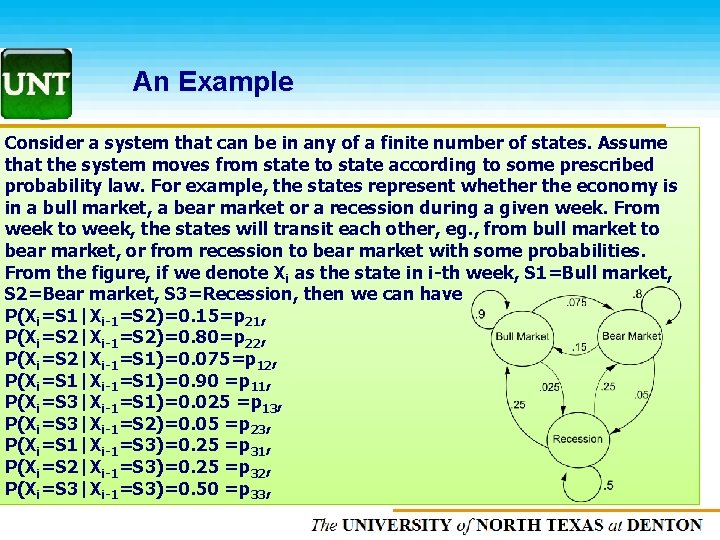
An Example Consider a system that can be in any of a finite number of states. Assume that the system moves from state to state according to some prescribed probability law. For example, the states represent whether the economy is in a bull market, a bear market or a recession during a given week. From week to week, the states will transit each other, eg. , from bull market to bear market, or from recession to bear market with some probabilities. From the figure, if we denote Xi as the state in i-th week, S 1=Bull market, S 2=Bear market, S 3=Recession, then we can have P(Xi=S 1|Xi-1=S 2)=0. 15=p 21, P(Xi=S 2|Xi-1=S 2)=0. 80=p 22, P(Xi=S 2|Xi-1=S 1)=0. 075=p 12, P(Xi=S 1|Xi-1=S 1)=0. 90 =p 11, P(Xi=S 3|Xi-1=S 1)=0. 025 =p 13, P(Xi=S 3|Xi-1=S 2)=0. 05 =p 23, P(Xi=S 1|Xi-1=S 3)=0. 25 =p 31, P(Xi=S 2|Xi-1=S 3)=0. 25 =p 32, P(Xi=S 3|Xi-1=S 3)=0. 50 =p 33, The UNIVERSITY of NORTH CAROLINA at CHAPEL HILL

Transition Matrix The UNIVERSITY of NORTH CAROLINA at CHAPEL HILL

Part 2. Formal Definitions The UNIVERSITY of NORTH CAROLINA at CHAPEL HILL

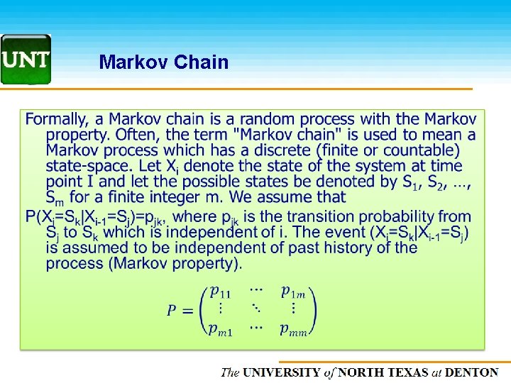
Markov Chain The UNIVERSITY of NORTH CAROLINA at CHAPEL HILL

Basic Operation: Probability after n steps Denote p(0)=[p 1(0), p 2(0), …, pm(0)] with pk(0)=P(X 0=Sk) where X 0 denote the starting state of the system. The p(n)=[p 1(n), …, pm(n)] is the probability after n steps. So we have p(1)=p(0)P, and p(n)=p(n-1)P Where P is the transition matrix. If P is regular, then there is a limit π=(π1, …, πm)=limn ∞p(n), which satisfies π= πP. The UNIVERSITY of NORTH CAROLINA at CHAPEL HILL

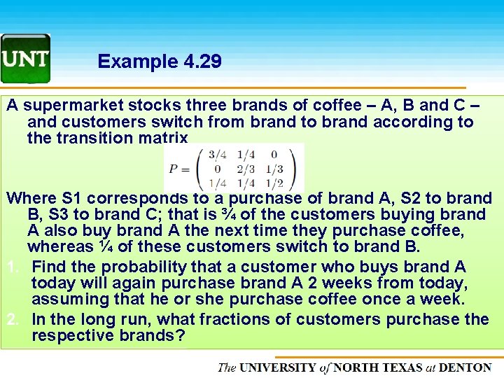
Example 4. 29 A supermarket stocks three brands of coffee – A, B and C – and customers switch from brand to brand according to the transition matrix Where S 1 corresponds to a purchase of brand A, S 2 to brand B, S 3 to brand C; that is ¾ of the customers buying brand A also buy brand A the next time they purchase coffee, whereas ¼ of these customers switch to brand B. 1. Find the probability that a customer who buys brand A today will again purchase brand A 2 weeks from today, assuming that he or she purchase coffee once a week. 2. In the long run, what fractions of customers purchase the respective brands? The UNIVERSITY of NORTH CAROLINA at CHAPEL HILL

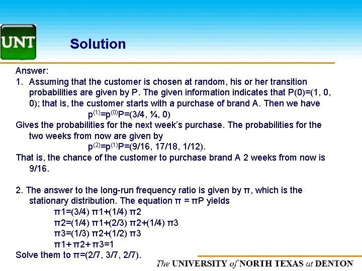
Solution Answer: 1. Assuming that the customer is chosen at random, his or her transition probabilities are given by P. The given information indicates that P(0)=(1, 0, 0); that is, the customer starts with a purchase of brand A. Then we have p(1)=p(0)P=(3/4, ¼, 0) Gives the probabilities for the next week’s purchase. The probabilities for the two weeks from now are given by p(2)=p(1)P=(9/16, 17/18, 1/12). That is, the chance of the customer to purchase brand A 2 weeks from now is 9/16. 2. The answer to the long-run frequency ratio is given by π, which is the stationary distribution. The equation π = πP yields π1=(3/4) π1+(1/4) π2 π2=(1/4) π1+(2/3) π2+(1/4) π3 π3=(1/3) π2+(1/2) π3 π1+ π2+ π3=1 Solve them to π=(2/7, 3/7, 2/7). The UNIVERSITY of NORTH CAROLINA at CHAPEL HILL

Chapter 5. Continuous Probability Distributions Section 5. 1: Continuous Random Variables and Their Probability Distributions Jiaping Wang Department of Mathematical Science 03/18/2013, Monday The UNIVERSITY of NORTH CAROLINA at CHAPEL HILL

Outline Introduction Density Function Distribution Function More Examples The UNIVERSITY of NORTH CAROLINA at CHAPEL HILL

Part 1. Introduction The UNIVERSITY of NORTH CAROLINA at CHAPEL HILL

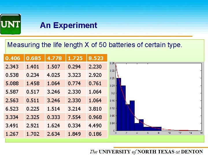
An Experiment Measuring the life length X of 50 batteries of certain type. 0. 406 0. 685 4. 778 1. 725 8. 523 2. 343 1. 401 1. 507 0. 294 2. 230 0. 538 0. 234 4. 025 3. 323 2. 920 5. 088 1. 458 1. 064 0. 774 0. 761 5. 587 0. 517 3. 246 2. 330 1. 064 2. 563 0. 511 3. 246 2. 330 1. 064 6. 523 0. 225 1. 514 3. 214 3. 810 3. 334 2. 325 0. 333 7. 554 0. 968 3. 491 2. 921 1. 624 0. 334 4. 490 1. 267 1. 702 2. 634 1. 849 0. 186 The UNIVERSITY of NORTH CAROLINA at CHAPEL HILL

Part 2. Density Function The UNIVERSITY of NORTH CAROLINA at CHAPEL HILL

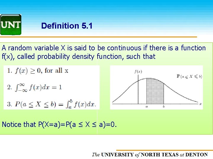
Definition 5. 1 A random variable X is said to be continuous if there is a function f(x), called probability density function, such that Notice that P(X=a)=P(a ≤ X ≤ a)=0. The UNIVERSITY of NORTH CAROLINA at CHAPEL HILL

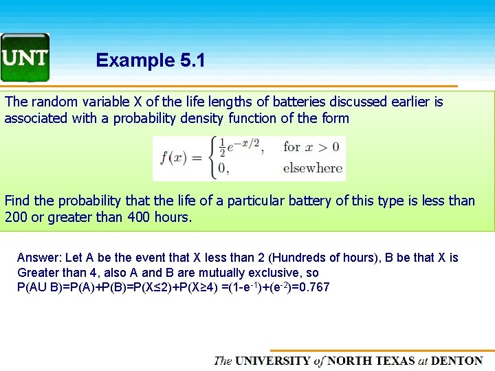
Example 5. 1 The random variable X of the life lengths of batteries discussed earlier is associated with a probability density function of the form Find the probability that the life of a particular battery of this type is less than 200 or greater than 400 hours. Answer: Let A be the event that X less than 2 (Hundreds of hours), B be that X is Greater than 4, also A and B are mutually exclusive, so P(AU B)=P(A)+P(B)=P(X≤ 2)+P(X≥ 4) =(1 -e-1)+(e-2)=0. 767 The UNIVERSITY of NORTH CAROLINA at CHAPEL HILL

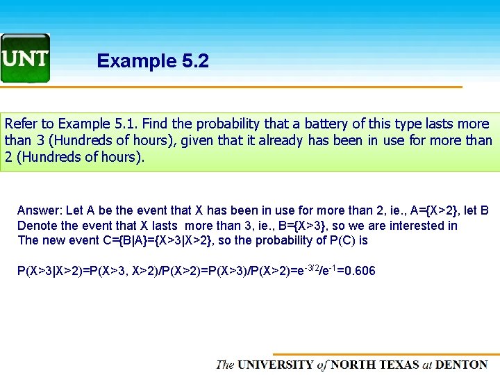
Example 5. 2 Refer to Example 5. 1. Find the probability that a battery of this type lasts more than 3 (Hundreds of hours), given that it already has been in use for more than 2 (Hundreds of hours). Answer: Let A be the event that X has been in use for more than 2, ie. , A={X>2}, let B Denote the event that X lasts more than 3, ie. , B={X>3}, so we are interested in The new event C={B|A}={X>3|X>2}, so the probability of P(C) is P(X>3|X>2)=P(X>3, X>2)/P(X>2)=P(X>3)/P(X>2)=e-3/2/e-1=0. 606 The UNIVERSITY of NORTH CAROLINA at CHAPEL HILL

Part 3. Distribution Function The UNIVERSITY of NORTH CAROLINA at CHAPEL HILL

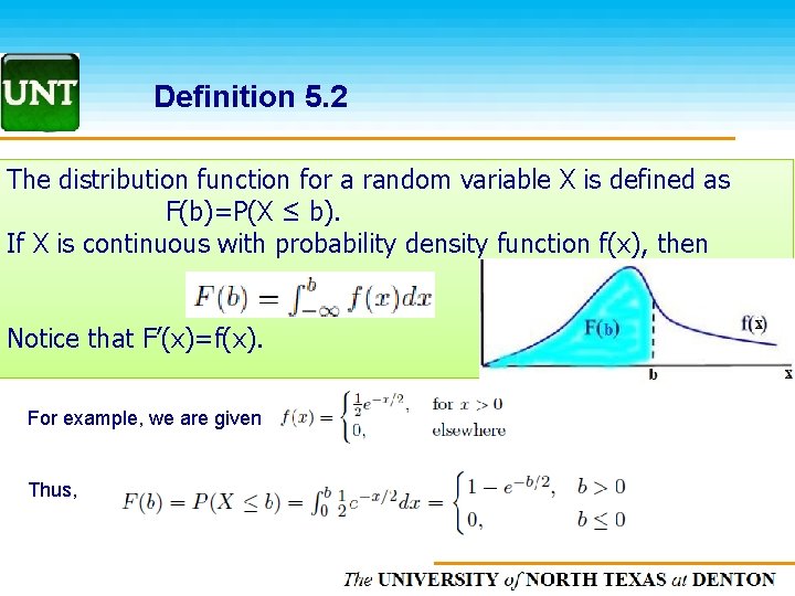
Definition 5. 2 The distribution function for a random variable X is defined as F(b)=P(X ≤ b). If X is continuous with probability density function f(x), then Notice that F’(x)=f(x). For example, we are given Thus, The UNIVERSITY of NORTH CAROLINA at CHAPEL HILL

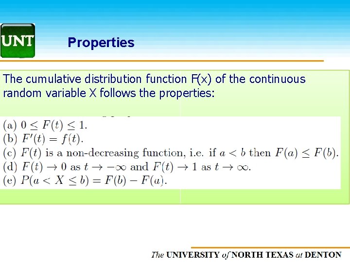
Properties The cumulative distribution function F(x) of the continuous random variable X follows the properties: The UNIVERSITY of NORTH CAROLINA at CHAPEL HILL

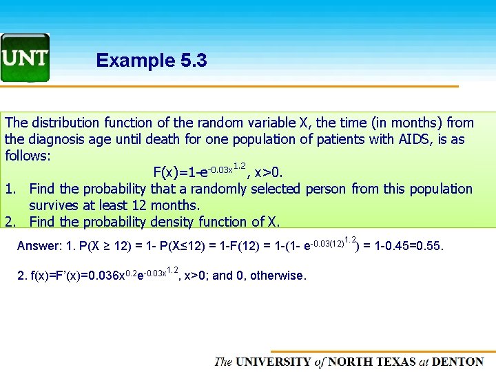
Example 5. 3 The distribution function of the random variable X, the time (in months) from the diagnosis age until death for one population of patients with AIDS, is as follows: 1. 2 F(x)=1 -e-0. 03 x , x>0. 1. Find the probability that a randomly selected person from this population survives at least 12 months. 2. Find the probability density function of X. 1. 2 Answer: 1. P(X ≥ 12) = 1 - P(X≤ 12) = 1 -F(12) = 1 -(1 - e-0. 03(12) ) = 1 -0. 45=0. 55. 1. 2 2. f(x)=F’(x)=0. 036 x 0. 2 e-0. 03 x , x>0; and 0, otherwise. The UNIVERSITY of NORTH CAROLINA at CHAPEL HILL

Part 3. More Examples The UNIVERSITY of NORTH CAROLINA at CHAPEL HILL

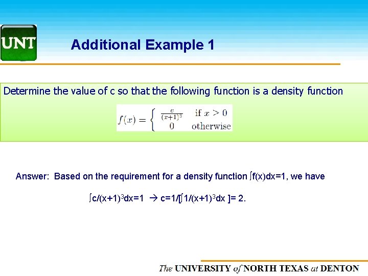
Additional Example 1 Determine the value of c so that the following function is a density function Answer: Based on the requirement for a density function ∫f(x)dx=1, we have ∫c/(x+1)3 dx=1 c=1/[∫ 1/(x+1)3 dx ]= 2. The UNIVERSITY of NORTH CAROLINA at CHAPEL HILL

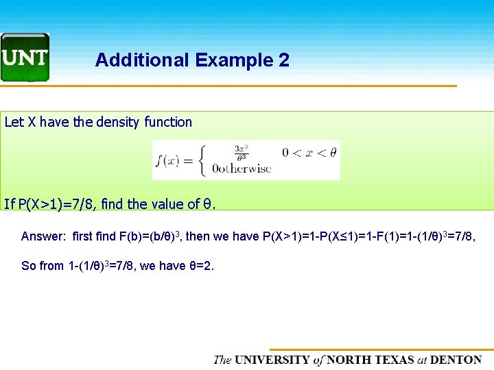
Additional Example 2 Let X have the density function If P(X>1)=7/8, find the value of θ. Answer: first find F(b)=(b/θ)3, then we have P(X>1)=1 -P(X≤ 1)=1 -F(1)=1 -(1/θ)3=7/8, So from 1 -(1/θ)3=7/8, we have θ=2. The UNIVERSITY of NORTH CAROLINA at CHAPEL HILL