Chapter 4 Discrete Probability Distributions 1 Chapter Outline

Chapter 4 Discrete Probability Distributions 1

Chapter Outline • 4. 1 Probability Distributions • 4. 2 Binomial Distributions • 4. 3 More Discrete Probability Distributions 2

Section 4. 1 Probability Distributions 3

Section 4. 1 Objectives • Distinguish between discrete random variables and continuous random variables • Construct a discrete probability distribution and its graph • Determine if a distribution is a probability distribution • Find the mean, variance, and standard deviation of a discrete probability distribution • Find the expected value of a discrete probability distribution 4

Random Variables Random Variable • Represents a numerical value associated with each outcome of a probability distribution. • Denoted by x • Examples § x = Number of sales calls a salesperson makes in one day. § x = Hours spent on sales calls in one day. 5

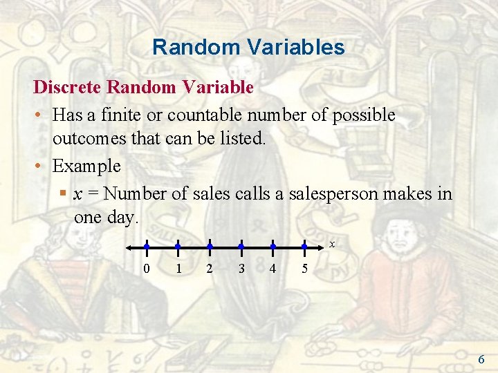
Random Variables Discrete Random Variable • Has a finite or countable number of possible outcomes that can be listed. • Example § x = Number of sales calls a salesperson makes in one day. x 0 1 2 3 4 5 6

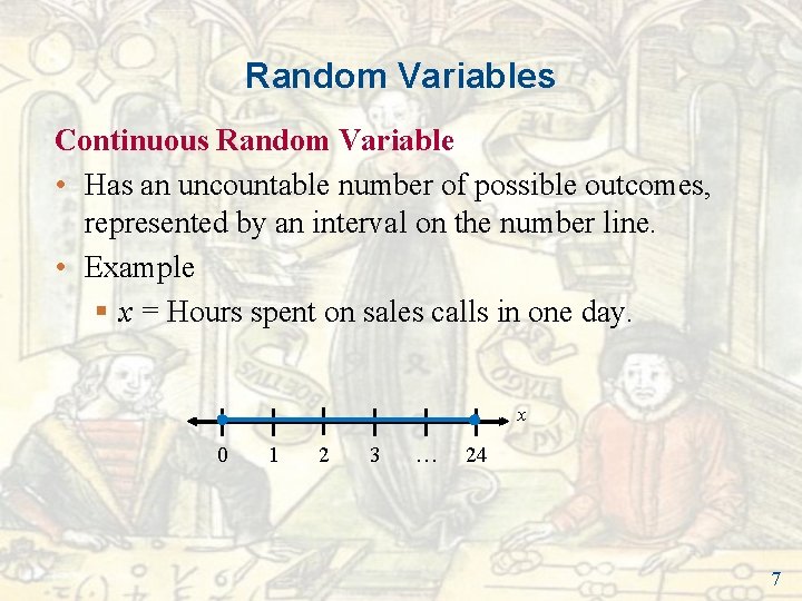
Random Variables Continuous Random Variable • Has an uncountable number of possible outcomes, represented by an interval on the number line. • Example § x = Hours spent on sales calls in one day. x 0 1 2 3 … 24 7

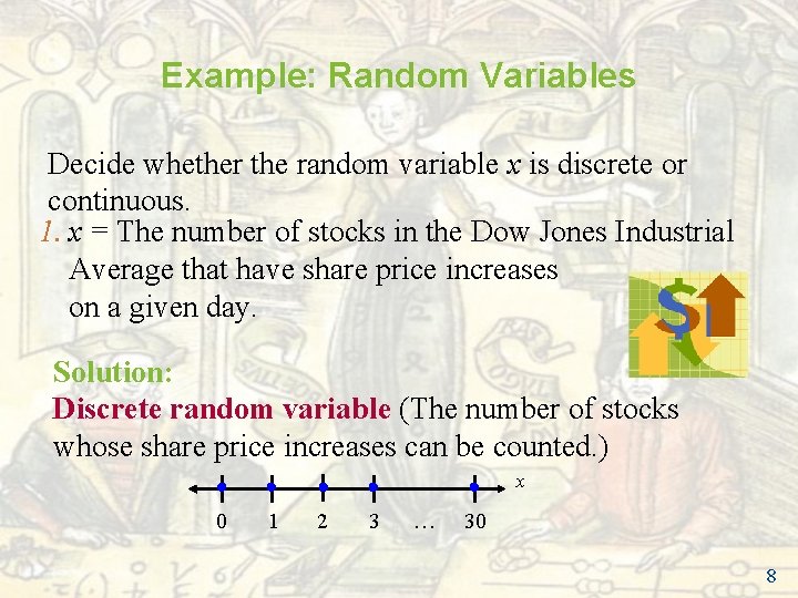
Example: Random Variables Decide whether the random variable x is discrete or continuous. 1. x = The number of stocks in the Dow Jones Industrial Average that have share price increases on a given day. Solution: Discrete random variable (The number of stocks whose share price increases can be counted. ) x 0 1 2 3 … 30 8

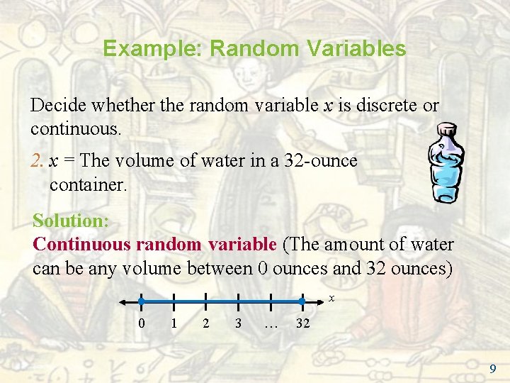
Example: Random Variables Decide whether the random variable x is discrete or continuous. 2. x = The volume of water in a 32 -ounce container. Solution: Continuous random variable (The amount of water can be any volume between 0 ounces and 32 ounces) x 0 1 2 3 … 32 9

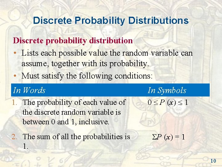
Discrete Probability Distributions Discrete probability distribution • Lists each possible value the random variable can assume, together with its probability. • Must satisfy the following conditions: In Words In Symbols 1. The probability of each value of the discrete random variable is between 0 and 1, inclusive. 0 P (x) 1 2. The sum of all the probabilities is 1. ΣP (x) = 1 10

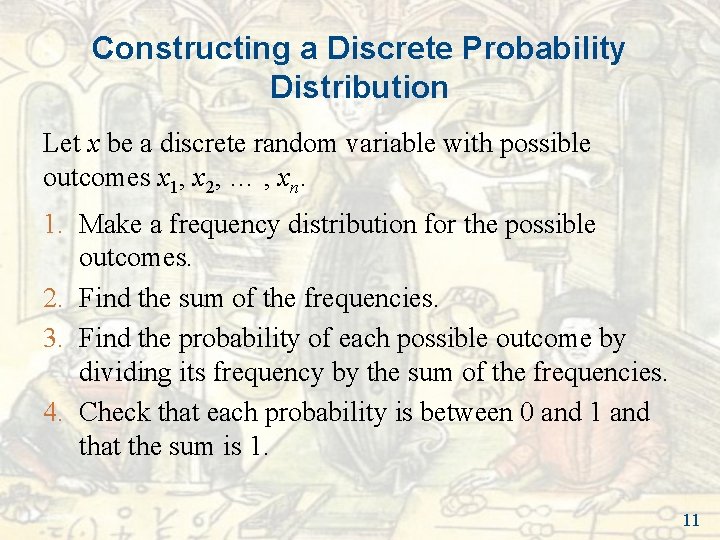
Constructing a Discrete Probability Distribution Let x be a discrete random variable with possible outcomes x 1, x 2, … , xn. 1. Make a frequency distribution for the possible outcomes. 2. Find the sum of the frequencies. 3. Find the probability of each possible outcome by dividing its frequency by the sum of the frequencies. 4. Check that each probability is between 0 and 1 and that the sum is 1. 11

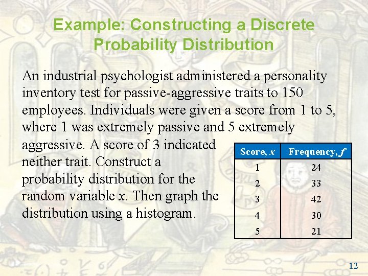
Example: Constructing a Discrete Probability Distribution An industrial psychologist administered a personality inventory test for passive-aggressive traits to 150 employees. Individuals were given a score from 1 to 5, where 1 was extremely passive and 5 extremely aggressive. A score of 3 indicated Score, x Frequency, f neither trait. Construct a 1 24 probability distribution for the 2 33 random variable x. Then graph the 3 42 distribution using a histogram. 4 30 5 21 12

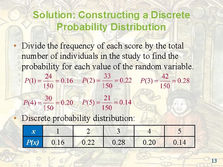
Solution: Constructing a Discrete Probability Distribution • Divide the frequency of each score by the total number of individuals in the study to find the probability for each value of the random variable. • Discrete probability distribution: x P(x) 1 0. 16 2 0. 22 3 0. 28 4 0. 20 5 0. 14 13

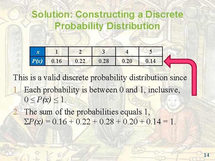
Solution: Constructing a Discrete Probability Distribution x 1 2 3 4 5 P(x) 0. 16 0. 22 0. 28 0. 20 0. 14 This is a valid discrete probability distribution since 1. Each probability is between 0 and 1, inclusive, 0 ≤ P(x) ≤ 1. 2. The sum of the probabilities equals 1, ΣP(x) = 0. 16 + 0. 22 + 0. 28 + 0. 20 + 0. 14 = 1. 14

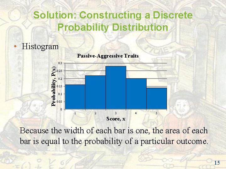
Solution: Constructing a Discrete Probability Distribution • Histogram Passive-Aggressive Traits Probability, P(x) 0. 3 0. 25 0. 2 0. 15 0. 1 0. 05 0 1 2 3 4 5 Score, x Because the width of each bar is one, the area of each bar is equal to the probability of a particular outcome. 15

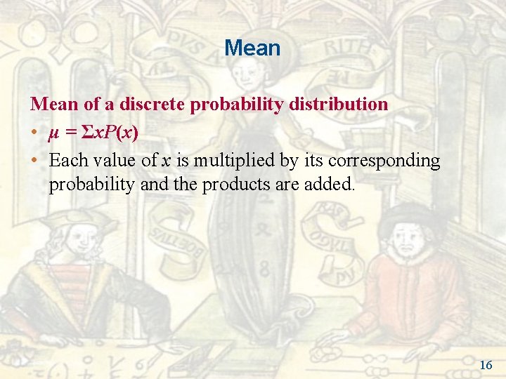
Mean of a discrete probability distribution • μ = Σx. P(x) • Each value of x is multiplied by its corresponding probability and the products are added. 16

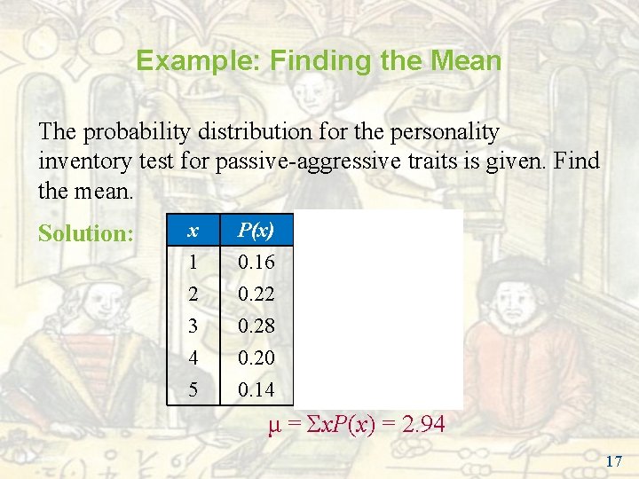
Example: Finding the Mean The probability distribution for the personality inventory test for passive-aggressive traits is given. Find the mean. Solution: x 1 2 3 P(x) 0. 16 0. 22 0. 28 x. P(x) 1(0. 16) = 0. 16 2(0. 22) = 0. 44 3(0. 28) = 0. 84 4 5 0. 20 0. 14 4(0. 20) = 0. 80 5(0. 14) = 0. 70 μ = Σx. P(x) = 2. 94 17

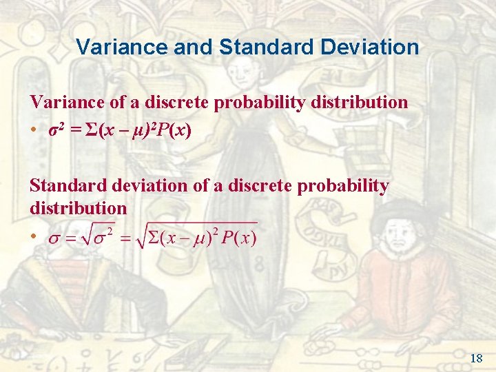
Variance and Standard Deviation Variance of a discrete probability distribution • σ2 = Σ(x – μ)2 P(x) Standard deviation of a discrete probability distribution • 18

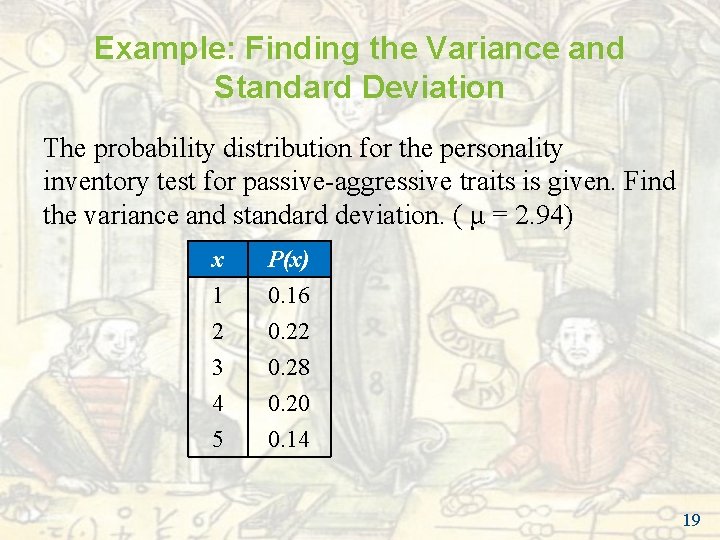
Example: Finding the Variance and Standard Deviation The probability distribution for the personality inventory test for passive-aggressive traits is given. Find the variance and standard deviation. ( μ = 2. 94) x 1 2 3 P(x) 0. 16 0. 22 0. 28 4 5 0. 20 0. 14 19

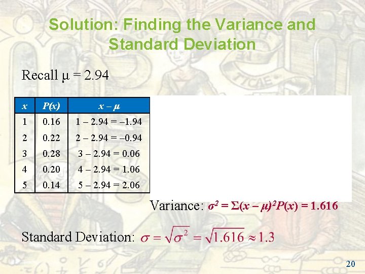
Solution: Finding the Variance and Standard Deviation Recall μ = 2. 94 x P(x) x–μ (x – μ)2 P(x) 1 0. 16 1 – 2. 94 = – 1. 94 (– 1. 94)2 = 3. 764(0. 16) = 0. 602 2 0. 22 2 – 2. 94 = – 0. 94 (– 0. 94)2 = 0. 884(0. 22) = 0. 194 3 0. 28 3 – 2. 94 = 0. 06 (0. 06)2 = 0. 004(0. 28) = 0. 001 4 0. 20 4 – 2. 94 = 1. 06 (1. 06)2 = 1. 124(0. 20) = 0. 225 5 0. 14 5 – 2. 94 = 2. 06 (2. 06)2 = 4. 244(0. 14) = 0. 594 Variance: σ2 = Σ(x – μ)2 P(x) = 1. 616 Standard Deviation: 20

Expected Value Expected value of a discrete random variable • Equal to the mean of the random variable. • E(x) = μ = Σx. P(x) 21

Example: Finding an Expected Value At a raffle, 1500 tickets are sold at $2 each for four prizes of $500, $250, $150, and $75. You buy one ticket. What is the expected value of your gain? 22

Solution: Finding an Expected Value • To find the gain for each prize, subtract the price of the ticket from the prize: § Your gain for the $500 prize is $500 – $2 = $498 § Your gain for the $250 prize is $250 – $2 = $248 § Your gain for the $150 prize is $150 – $2 = $148 § Your gain for the $75 prize is $75 – $2 = $73 • If you do not win a prize, your gain is $0 – $2 = –$2 23

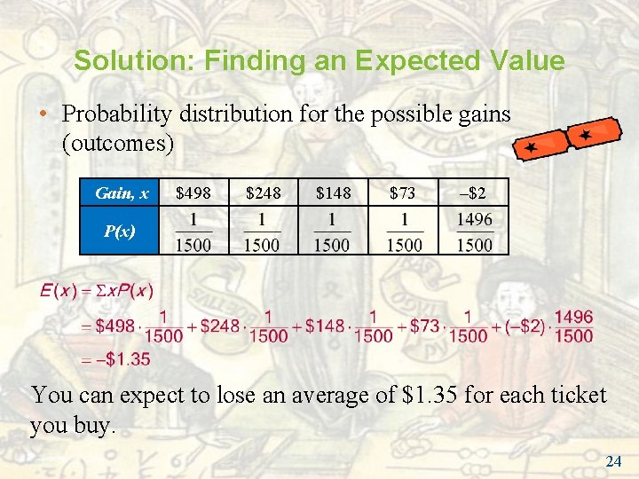
Solution: Finding an Expected Value • Probability distribution for the possible gains (outcomes) Gain, x $498 $248 $148 $73 –$2 P(x) You can expect to lose an average of $1. 35 for each ticket you buy. 24

Section 4. 1 Summary • Distinguished between discrete random variables and continuous random variables • Constructed a discrete probability distribution and its graph • Determined if a distribution is a probability distribution • Found the mean, variance, and standard deviation of a discrete probability distribution • Found the expected value of a discrete probability distribution 25

Random Variables http: //www. learner. org/courses/againstallodds/unitpages/unit 20. html. Slide 4 - 26

Section 4. 2 Binomial Distributions 27

Section 4. 2 Objectives • Determine if a probability experiment is a binomial experiment • Find binomial probabilities using the binomial probability formula • Find binomial probabilities using technology and a binomial table • Graph a binomial distribution • Find the mean, variance, and standard deviation of a binomial probability distribution 28

Binomial Experiments 1. The experiment is repeated for a fixed number of trials, where each trial is independent of other trials. 2. There are only two possible outcomes of interest for each trial. The outcomes can be classified as a success (S) or as a failure (F). 3. The probability of a success P(S) is the same for each trial. 4. The random variable x counts the number of successful trials. 29

Notation for Binomial Experiments Symbol n p = P(s) q = P(F) x Description The number of times a trial is repeated The probability of success in a single trial The probability of failure in a single trial (q = 1 – p) The random variable represents a count of the number of successes in n trials: x = 0, 1, 2, 3, … , n. 30

Example: Binomial Experiments Decide whether the experiment is a binomial experiment. If it is, specify the values of n, p, and q, and list the possible values of the random variable x. 1. A certain surgical procedure has an 85% chance of success. A doctor performs the procedure on eight patients. The random variable represents the number of successful surgeries. 31

Solution: Binomial Experiments Binomial Experiment 1. Each surgery represents a trial. There are eight surgeries, and each one is independent of the others. 2. There are only two possible outcomes of interest for each surgery: a success (S) or a failure (F). 3. The probability of a success, P(S), is 0. 85 for each surgery. 4. The random variable x counts the number of successful surgeries. 32

Solution: Binomial Experiments Binomial Experiment • n = 8 (number of trials) • p = 0. 85 (probability of success) • q = 1 – p = 1 – 0. 85 = 0. 15 (probability of failure) • x = 0, 1, 2, 3, 4, 5, 6, 7, 8 (number of successful surgeries) 33

Example: Binomial Experiments Decide whether the experiment is a binomial experiment. If it is, specify the values of n, p, and q, and list the possible values of the random variable x. 2. A jar contains five red marbles, nine blue marbles, and six green marbles. You randomly select three marbles from the jar, without replacement. The random variable represents the number of red marbles. 34

Solution: Binomial Experiments Not a Binomial Experiment • The probability of selecting a red marble on the first trial is 5/20. • Because the marble is not replaced, the probability of success (red) for subsequent trials is no longer 5/20. • The trials are not independent and the probability of a success is not the same for each trial. 35

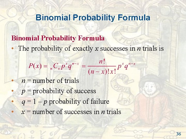
Binomial Probability Formula • The probability of exactly x successes in n trials is • • n = number of trials p = probability of success q = 1 – p probability of failure x = number of successes in n trials 36

Example: Finding Binomial Probabilities Microfracture knee surgery has a 75% chance of success on patients with degenerative knees. The surgery is performed on three patients. Find the probability of the surgery being successful on exactly two patients. 37

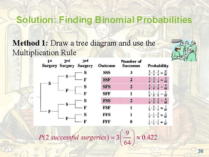
Solution: Finding Binomial Probabilities Method 1: Draw a tree diagram and use the Multiplication Rule 38

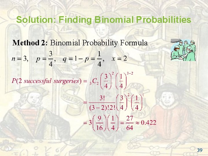
Solution: Finding Binomial Probabilities Method 2: Binomial Probability Formula 39

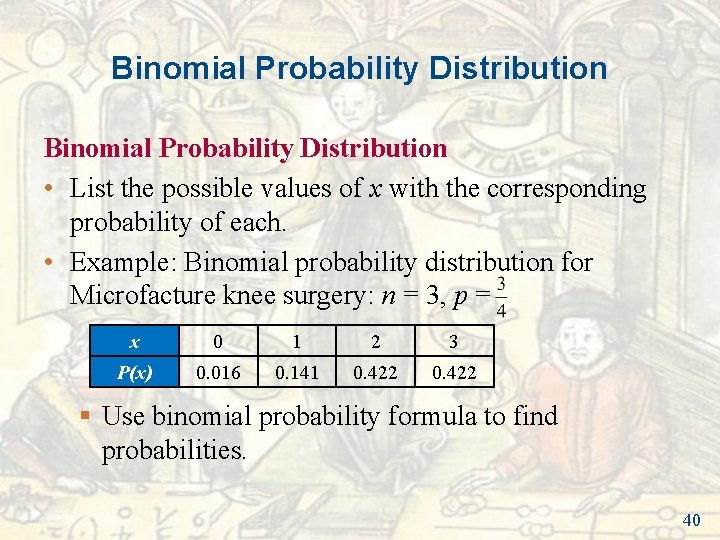
Binomial Probability Distribution • List the possible values of x with the corresponding probability of each. • Example: Binomial probability distribution for Microfacture knee surgery: n = 3, p = x 0 1 2 3 P(x) 0. 016 0. 141 0. 422 § Use binomial probability formula to find probabilities. 40

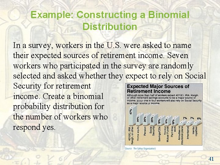
Example: Constructing a Binomial Distribution In a survey, workers in the U. S. were asked to name their expected sources of retirement income. Seven workers who participated in the survey are randomly selected and asked whether they expect to rely on Social Security for retirement income. Create a binomial probability distribution for the number of workers who respond yes. 41

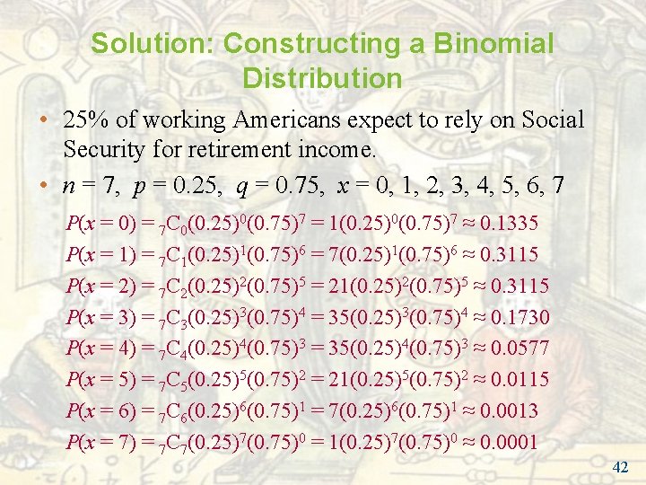
Solution: Constructing a Binomial Distribution • 25% of working Americans expect to rely on Social Security for retirement income. • n = 7, p = 0. 25, q = 0. 75, x = 0, 1, 2, 3, 4, 5, 6, 7 P(x = 0) = 7 C 0(0. 25)0(0. 75)7 = 1(0. 25)0(0. 75)7 ≈ 0. 1335 P(x = 1) = 7 C 1(0. 25)1(0. 75)6 = 7(0. 25)1(0. 75)6 ≈ 0. 3115 P(x = 2) = 7 C 2(0. 25)2(0. 75)5 = 21(0. 25)2(0. 75)5 ≈ 0. 3115 P(x = 3) = 7 C 3(0. 25)3(0. 75)4 = 35(0. 25)3(0. 75)4 ≈ 0. 1730 P(x = 4) = 7 C 4(0. 25)4(0. 75)3 = 35(0. 25)4(0. 75)3 ≈ 0. 0577 P(x = 5) = 7 C 5(0. 25)5(0. 75)2 = 21(0. 25)5(0. 75)2 ≈ 0. 0115 P(x = 6) = 7 C 6(0. 25)6(0. 75)1 = 7(0. 25)6(0. 75)1 ≈ 0. 0013 P(x = 7) = 7 C 7(0. 25)7(0. 75)0 = 1(0. 25)7(0. 75)0 ≈ 0. 0001 42

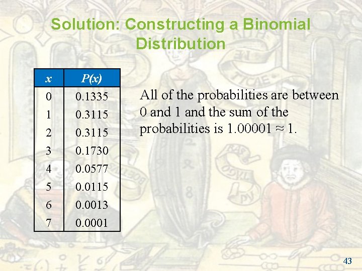
Solution: Constructing a Binomial Distribution x 0 1 2 P(x) 0. 1335 0. 3115 3 4 5 6 7 0. 1730 0. 0577 0. 0115 0. 0013 0. 0001 All of the probabilities are between 0 and 1 and the sum of the probabilities is 1. 00001 ≈ 1. 43

Example: Finding Binomial Probabilities A survey indicates that 41% of women in the U. S. consider reading their favorite leisure-time activity. You randomly select four U. S. women and ask them if reading is their favorite leisure-time activity. Find the probability that at least two of them respond yes. Solution: • n = 4, p = 0. 41, q = 0. 59 • At least two means two or more. • Find the sum of P(2), P(3), and P(4). 44

Solution: Finding Binomial Probabilities P(x = 2) = 4 C 2(0. 41)2(0. 59)2 = 6(0. 41)2(0. 59)2 ≈ 0. 351094 P(x = 3) = 4 C 3(0. 41)3(0. 59)1 = 4(0. 41)3(0. 59)1 ≈ 0. 162654 P(x = 4) = 4 C 4(0. 41)4(0. 59)0 = 1(0. 41)4(0. 59)0 ≈ 0. 028258 P(x ≥ 2) = P(2) + P(3) + P(4) ≈ 0. 351094 + 0. 162654 + 0. 028258 ≈ 0. 542 45

Example: Finding Binomial Probabilities Using Technology The results of a recent survey indicate that when grilling, 59% of households in the United States use a gas grill. If you randomly select 100 households, what is the probability that exactly 65 households use a gas grill? Use a technology tool to find the probability. (Source: Greenfield Online for Weber-Stephens Products Company) Solution: • Binomial with n = 100, p = 0. 59, x = 65 46

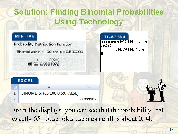
Solution: Finding Binomial Probabilities Using Technology From the displays, you can see that the probability that exactly 65 households use a gas grill is about 0. 04. 47

Example: Finding Binomial Probabilities Using a Table About thirty percent of working adults spend less than 15 minutes each way commuting to their jobs. You randomly select six working adults. What is the probability that exactly three of them spend less than 15 minutes each way commuting to work? Use a table to find the probability. (Source: U. S. Census Bureau) Solution: • Binomial with n = 6, p = 0. 30, x = 3 48

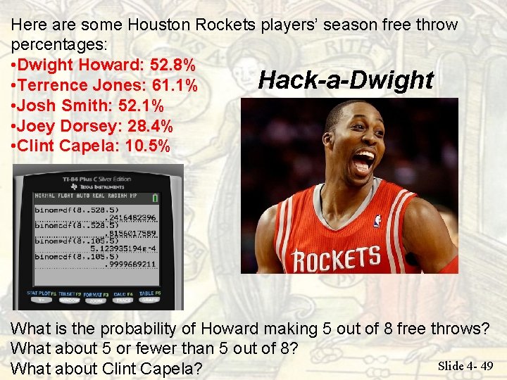
Here are some Houston Rockets players’ season free throw percentages: • Dwight Howard: 52. 8% Hack-a-Dwight • Terrence Jones: 61. 1% • Josh Smith: 52. 1% • Joey Dorsey: 28. 4% • Clint Capela: 10. 5% What is the probability of Howard making 5 out of 8 free throws? What about 5 or fewer than 5 out of 8? . Slide 4 - 49 What about Clint Capela?

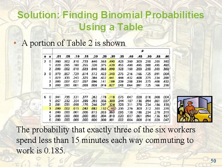
Solution: Finding Binomial Probabilities Using a Table • A portion of Table 2 is shown The probability that exactly three of the six workers spend less than 15 minutes each way commuting to work is 0. 185. 50

Example: Graphing a Binomial Distribution Fifty-nine percent of households in the U. S. subscribe to cable TV. You randomly select six households and ask each if they subscribe to cable TV. Construct a probability distribution for the random variable x. Then graph the distribution. (Source: Kagan Research, LLC) Solution: • n = 6, p = 0. 59, q = 0. 41 • Find the probability for each value of x 51

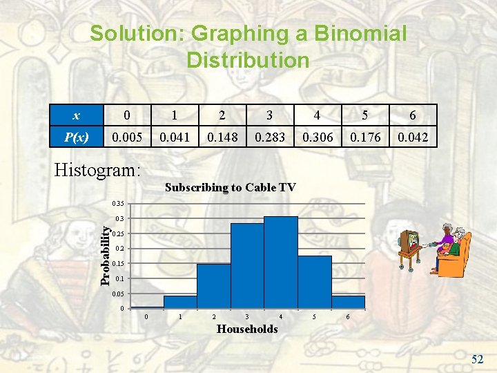
Solution: Graphing a Binomial Distribution x 0 1 2 3 4 5 6 P(x) 0. 005 0. 041 0. 148 0. 283 0. 306 0. 176 0. 042 Histogram: Subscribing to Cable TV 0. 35 Probability 0. 3 0. 25 0. 2 0. 15 0. 1 0. 05 0 0 1 2 3 4 5 6 Households 52

Binomial Distributions http: //www. learner. org/courses/againstallodds/unitpages/unit 21. html. Slide 4 - 53

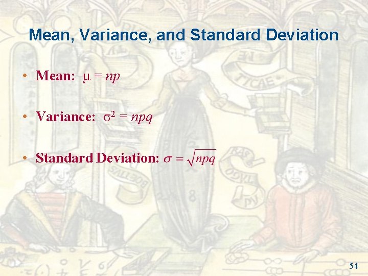
Mean, Variance, and Standard Deviation • Mean: μ = np • Variance: σ2 = npq • Standard Deviation: 54

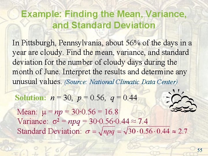
Example: Finding the Mean, Variance, and Standard Deviation In Pittsburgh, Pennsylvania, about 56% of the days in a year are cloudy. Find the mean, variance, and standard deviation for the number of cloudy days during the month of June. Interpret the results and determine any unusual values. (Source: National Climatic Data Center) Solution: n = 30, p = 0. 56, q = 0. 44 Mean: μ = np = 30∙ 0. 56 = 16. 8 Variance: σ2 = npq = 30∙ 0. 56∙ 0. 44 ≈ 7. 4 Standard Deviation: 55

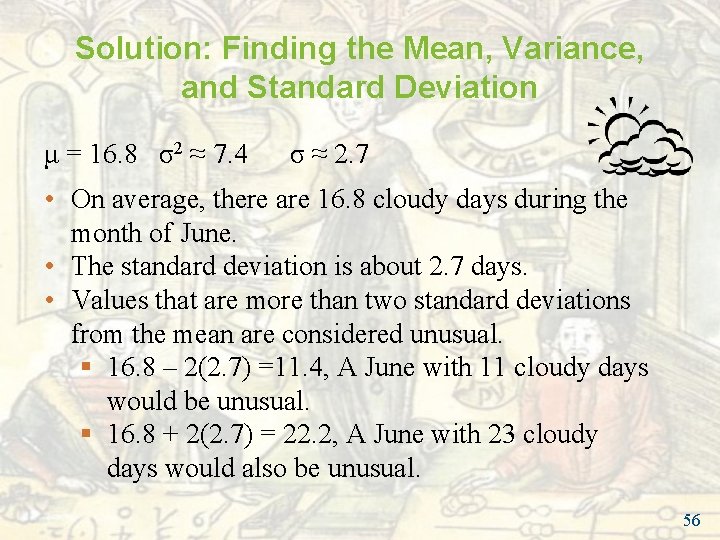
Solution: Finding the Mean, Variance, and Standard Deviation μ = 16. 8 σ2 ≈ 7. 4 σ ≈ 2. 7 • On average, there are 16. 8 cloudy days during the month of June. • The standard deviation is about 2. 7 days. • Values that are more than two standard deviations from the mean are considered unusual. § 16. 8 – 2(2. 7) =11. 4, A June with 11 cloudy days would be unusual. § 16. 8 + 2(2. 7) = 22. 2, A June with 23 cloudy days would also be unusual. 56

Section 4. 2 Summary • Determined if a probability experiment is a binomial experiment • Found binomial probabilities using the binomial probability formula • Found binomial probabilities using technology and a binomial table • Graphed a binomial distribution • Found the mean, variance, and standard deviation of a binomial probability distribution 57

Section 4. 3 More Discrete Probability Distributions 58

Section 4. 3 Objectives • Find probabilities using the geometric distribution • Find probabilities using the Poisson distribution 59

Geometric Distribution Geometric distribution • A discrete probability distribution. • Satisfies the following conditions § A trial is repeated until a success occurs. § The repeated trials are independent of each other. § The probability of success p is constant for each trial. • The probability that the first success will occur on trial x is P(x) = p(q)x – 1, where q = 1 – p. 60

Example: Geometric Distribution From experience, you know that the probability that you will make a sale on any given telephone call is 0. 23. Find the probability that your first sale on any given day will occur on your fourth or fifth sales call. Solution: • P(sale on fourth or fifth call) = P(4) + P(5) • Geometric with p = 0. 23, q = 0. 77, x = 4, 5 61

Solution: Geometric Distribution • P(4) = 0. 23(0. 77)4– 1 ≈ 0. 105003 • P(5) = 0. 23(0. 77)5– 1 ≈ 0. 080852 P(sale on fourth or fifth call) = P(4) + P(5) ≈ 0. 105003 + 0. 080852 ≈ 0. 186 62

Poisson Distribution Poisson distribution • A discrete probability distribution. • Satisfies the following conditions § The experiment consists of counting the number of times an event, x, occurs in a given interval. The interval can be an interval of time, area, or volume. § The probability of the event occurring is the same for each interval. § The number of occurrences in one interval is independent of the number of occurrences in other intervals. 63

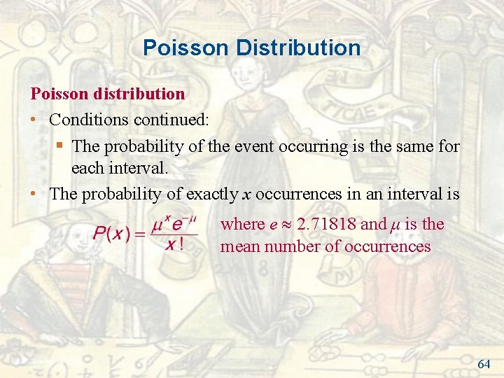
Poisson Distribution Poisson distribution • Conditions continued: § The probability of the event occurring is the same for each interval. • The probability of exactly x occurrences in an interval is where e 2. 71818 and μ is the mean number of occurrences 64

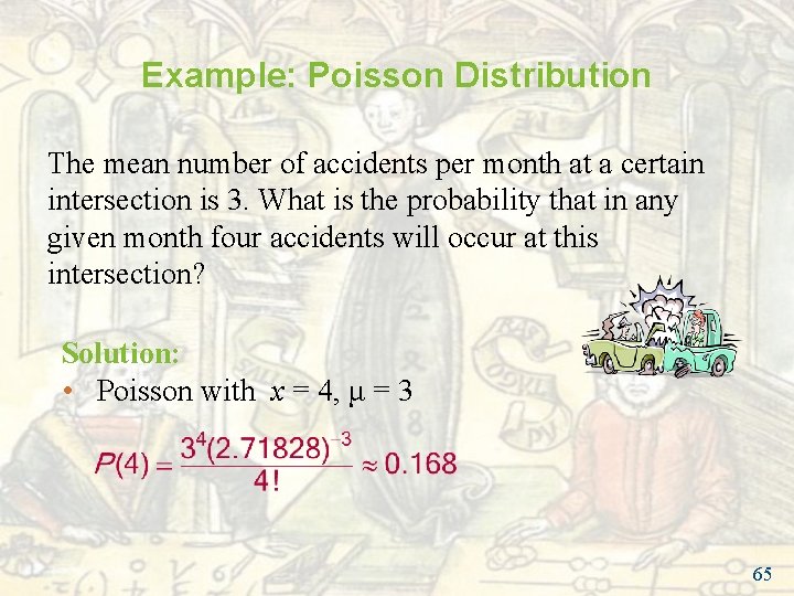
Example: Poisson Distribution The mean number of accidents per month at a certain intersection is 3. What is the probability that in any given month four accidents will occur at this intersection? Solution: • Poisson with x = 4, μ = 3 65

Section 4. 3 Summary • Found probabilities using the geometric distribution • Found probabilities using the Poisson distribution 66

Chapter 4: Discrete Probability Distributions Elementary Statistics: Picturing the World Fifth Edition by Larson and Farber . Slide 4 - 67

True or false: The number of kittens in a litter is an example of a discrete random variable. A. True B. False . Slide 4 - 68

True or false: The number of kittens in a litter is an example of a discrete random variable. A. True B. False . Slide 4 - 69

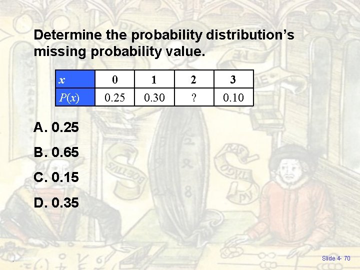
Determine the probability distribution’s missing probability value. x P(x) 0 0. 25 1 0. 30 2 ? 3 0. 10 A. 0. 25 B. 0. 65 C. 0. 15 D. 0. 35 . Slide 4 - 70

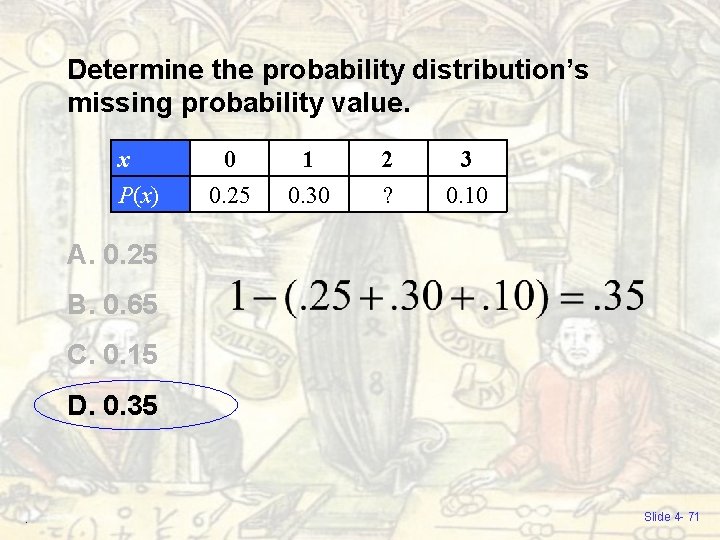
Determine the probability distribution’s missing probability value. x P(x) 0 0. 25 1 0. 30 2 ? 3 0. 10 A. 0. 25 B. 0. 65 C. 0. 15 D. 0. 35 . Slide 4 - 71

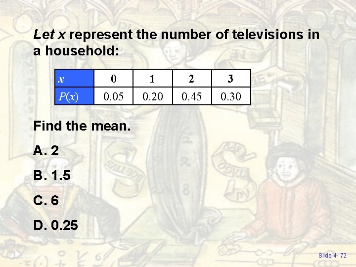
Let x represent the number of televisions in a household: x P(x) 0 0. 05 1 0. 20 2 0. 45 3 0. 30 Find the mean. A. 2 B. 1. 5 C. 6 D. 0. 25. Slide 4 - 72

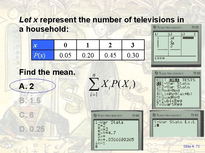
Let x represent the number of televisions in a household: x P(x) 0 0. 05 1 0. 20 2 0. 45 3 0. 30 Find the mean. A. 2 B. 1. 5 C. 6 D. 0. 25. Slide 4 - 73

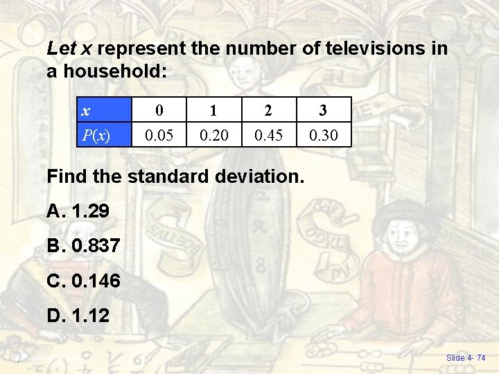
Let x represent the number of televisions in a household: x P(x) 0 0. 05 1 0. 20 2 0. 45 3 0. 30 Find the standard deviation. A. 1. 29 B. 0. 837 C. 0. 146 D. 1. 12. Slide 4 - 74

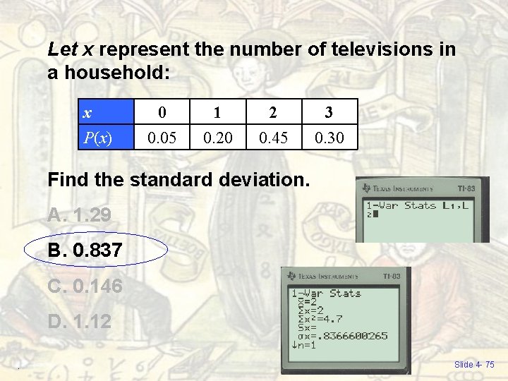
Let x represent the number of televisions in a household: x P(x) 0 0. 05 1 0. 20 2 0. 45 3 0. 30 Find the standard deviation. A. 1. 29 B. 0. 837 C. 0. 146 D. 1. 12. Slide 4 - 75

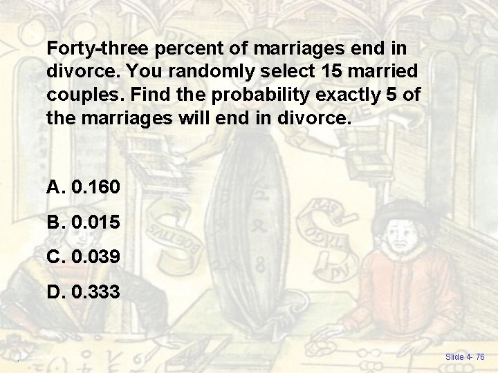
Forty-three percent of marriages end in divorce. You randomly select 15 married couples. Find the probability exactly 5 of the marriages will end in divorce. A. 0. 160 B. 0. 015 C. 0. 039 D. 0. 333 . Slide 4 - 76

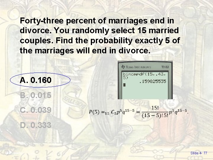
Forty-three percent of marriages end in divorce. You randomly select 15 married couples. Find the probability exactly 5 of the marriages will end in divorce. A. 0. 160 B. 0. 015 C. 0. 039 D. 0. 333 . Slide 4 - 77

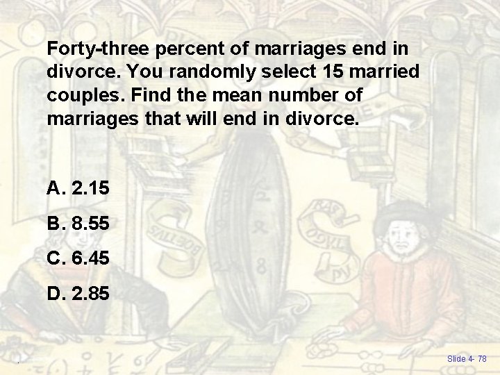
Forty-three percent of marriages end in divorce. You randomly select 15 married couples. Find the mean number of marriages that will end in divorce. A. 2. 15 B. 8. 55 C. 6. 45 D. 2. 85 . Slide 4 - 78

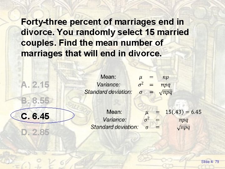
Forty-three percent of marriages end in divorce. You randomly select 15 married couples. Find the mean number of marriages that will end in divorce. A. 2. 15 B. 8. 55 C. 6. 45 D. 2. 85 . Slide 4 - 79

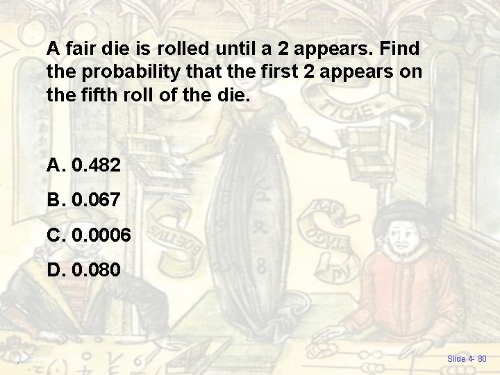
A fair die is rolled until a 2 appears. Find the probability that the first 2 appears on the fifth roll of the die. A. 0. 482 B. 0. 067 C. 0. 0006 D. 0. 080 . Slide 4 - 80

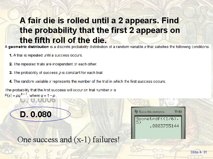
A fair die is rolled until a 2 appears. Find the probability that the first 2 appears on the fifth roll of the die. A. 0. 482 B. 0. 067 C. 0. 0006 D. 0. 080 One success and (x-1) failures! Slide 4 - 81

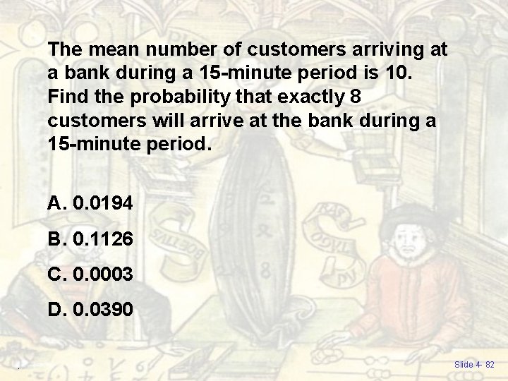
The mean number of customers arriving at a bank during a 15 -minute period is 10. Find the probability that exactly 8 customers will arrive at the bank during a 15 -minute period. A. 0. 0194 B. 0. 1126 C. 0. 0003 D. 0. 0390. Slide 4 - 82

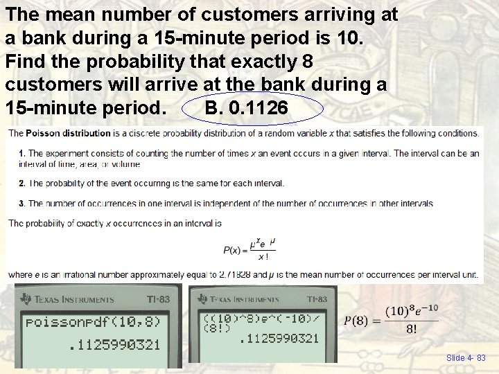
The mean number of customers arriving at a bank during a 15 -minute period is 10. Find the probability that exactly 8 customers will arrive at the bank during a 15 -minute period. B. 0. 1126 Slide 4 - 83