Chapter 4 Digital Transmission Mc GrawHill The Mc

Chapter 4 Digital Transmission Mc. Graw-Hill ©The Mc. Graw-Hill Companies, Inc. , 2004

Digital Transmission n Digital data to digital signal l n Analog data to digital signal l Mc. Graw-Hill Line coding PCM (Pulse code modulation) ©The Mc. Graw-Hill Companies, Inc. , 2004

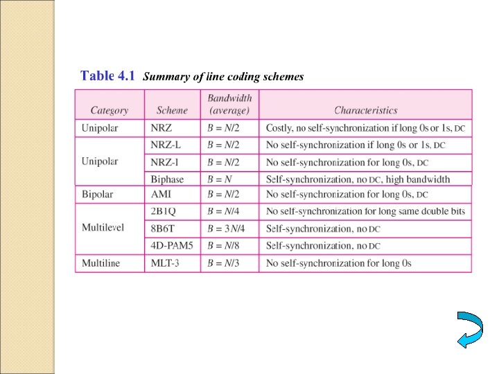
4. 1 Line Coding Some Characteristics Line Coding Schemes Some Other Schemes Mc. Graw-Hill ©The Mc. Graw-Hill Companies, Inc. , 2004

Figure 4. 1 Digital Transmission: Line coding Actual signal: digital pulse Digital data: Abstract Data n Mc. Graw-Hill วตถประสงคของการทำ Line coding n เพอแทน digital data ดวย ระดบ voltage ทกำหนด n เพอกำจดหรอลดปญหา n เพอเพมความเรวในการสงขอมล ©The Mc. Graw-Hill Companies, Inc. , 2004

Figure 4. 2 Signal level versus data level ‘ 1’: +5 V ‘ 0’: 0 V ‘ 1’: +5 V or -5 V ‘ 0’: 0 V + + two Mc. Graw-Hill ©The Mc. Graw-Hill Companies, Inc. , 2004

Figure 4. 3 DC component + + + + - Mc. Graw-Hill - - - ©The Mc. Graw-Hill Companies, Inc. , 2004

DC Component Problem สญญาณดจตอลทมองคประกอบ ทำใหระดบสญญาณเพยนไป DC Stray Capacitance Mc. Graw-Hill ©The Mc. Graw-Hill Companies, Inc. , 2004

Figure 4. 4 Lack of synchronization Fast clock Mc. Graw-Hill ©The Mc. Graw-Hill Companies, Inc. , 2004

Example 3 In a digital transmission, the receiver clock is 0. 1 percent faster than the sender clock. How many extra bits per second does the receiver receive if the data rate is 1 Kbps? How many if the data rate is 1 Mbps? Solution At 1 Kbps: 1000 bits sent 1001 bits received 1 extra bps At 1 Mbps: 1, 000 bits sent 1, 000 bits received 1000 extra bps Mc. Graw-Hill ©The Mc. Graw-Hill Companies, Inc. , 2004

Signal level (Element) versus Data level (Element)

Example 1 A signal has two data levels with a pulse duration of 1 ms. We calculate the pulse rate and bit rate as follows: Pulse duration = signal duration (sec) = 1 ms Pulse Rate = 1/ 10 -3= 1000 pulses/s L = data level L = 2; Bit Rate = Pulse Rate x log 2 L = 1000 x log 2 2 = 1000 bps L = 4; Bit Rate = 1000 x log 2 4 = 2000 bps Mc. Graw-Hill ©The Mc. Graw-Hill Companies, Inc. , 2004

Figure 4. 5 Line coding schemes Multi-level Mc. Graw-Hill ©The Mc. Graw-Hill Companies, Inc. , 2004

Figure 4. 6 Unipolar encoding Note: Unipolar encoding uses only one voltage level (positive or negative). + Mc. Graw-Hill + + + ©The Mc. Graw-Hill Companies, Inc. , 2004

Figure 4. 7 Types of polar encoding Note: Polar encoding uses two voltage levels (positive and negative). Mc. Graw-Hill ©The Mc. Graw-Hill Companies, Inc. , 2004

Note: In NRZ-L the level of the signal is dependent upon the state of the bit. In NRZ-I (NRZ-M) the signal is inverted if a 1 is encountered. Mc. Graw-Hill ©The Mc. Graw-Hill Companies, Inc. , 2004

Figure 4. 8 NRZ-L and NRZ-I encoding NRZ-L: Non-Return-to-Zero-Level ‘ 0’: +5 V ‘ 1’: -5 V NRZ-I: Non-Return-to-Zero-Inversion NRZ-M: Non-Return-to-Zero-Mark + + + - Mc. Graw-Hill - - + + ‘ 1’: Inversion ‘ 0’: Noninversion - ©The Mc. Graw-Hill Companies, Inc. , 2004

Figure 4. 9 Return-to-Zero (RZ) encoding Bipolar-Return-to-Zero (BIP) A good encoded digital signal must contain a provision for synchronization. ‘ 0’: ‘ 1’: Mc. Graw-Hill ©The Mc. Graw-Hill Companies, Inc. , 2004

Note: In Manchester encoding, the transition at the middle of the bit is used for both synchronization and bit representation. Mc. Graw-Hill ©The Mc. Graw-Hill Companies, Inc. , 2004

Figure 4. 10 Mc. Graw-Hill Manchester encoding ©The Mc. Graw-Hill Companies, Inc. , 2004

Note: In differential Manchester encoding, the transition at the middle of the bit is used only for synchronization. The bit representation is defined by the inversion or noninversion at the beginning of the bit. Mc. Graw-Hill ©The Mc. Graw-Hill Companies, Inc. , 2004

Figure 4. 11 Differential Manchester encoding ‘ 0’: Inversion ‘ 1’: Noninversion Mc. Graw-Hill ©The Mc. Graw-Hill Companies, Inc. , 2004

Figure 4. 12 Bipolar AMI encoding In bipolar encoding, we use three levels: positive, zero, and negative. ‘ 1’: Inversion ‘ 0’: 0 V Mc. Graw-Hill ©The Mc. Graw-Hill Companies, Inc. , 2004

Figure 5 -11 B 8 ZS Encoding Mc. Graw-Hill ©The Mc. Graw-Hill Companies, Inc. , 2004

Figure 5 -13 Example: B 8 ZS Encoding Mc. Graw-Hill ©The Mc. Graw-Hill Companies, Inc. , 2004

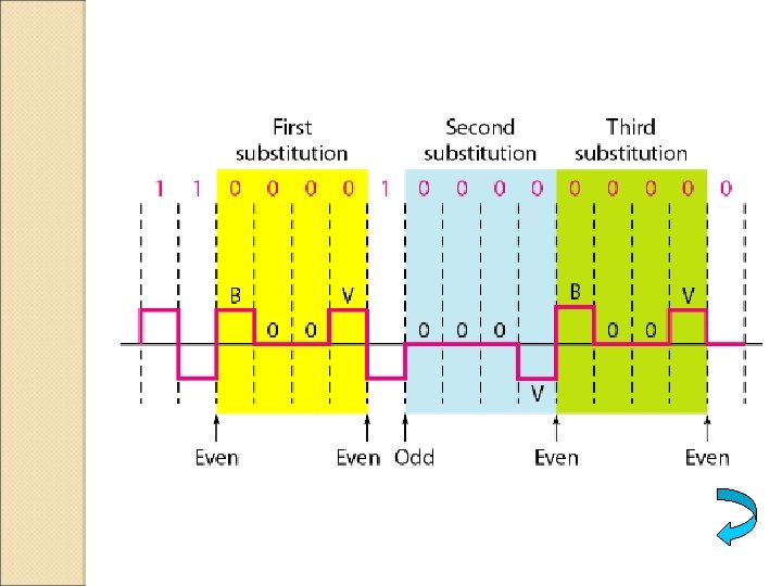
Figure 5 -12 HDB 3 Encoding Mc. Graw-Hill ©The Mc. Graw-Hill Companies, Inc. , 2004

Figure 5 -14 Example: HDB 3 Encoding Mc. Graw-Hill ©The Mc. Graw-Hill Companies, Inc. , 2004

Line Coding Multi-level coding 1) 2 B 1 Q 2) 8 B/6 T 3) MLT-3 Mc. Graw-Hill ©The Mc. Graw-Hill Companies, Inc. , 2000

Figure 4. 13 2 B 1 Q - Used in ISDN 64 kbps or 128 kbps via telephone line Mc. Graw-Hill ©The Mc. Graw-Hill Companies, Inc. , 2004

Figure 4. 17 Example of 8 B/6 T encoding Used in 100 BASET 4 Ethernet (100 Mbps) via UTP in Star Topology Mc. Graw-Hill ©The Mc. Graw-Hill Companies, Inc. , 2004

‘ 0’: Inversion ‘ 1’: Noninversion ( -V, 0, +V) First introduced by Cisco System for FDDI (Fiber Distributed Data Interface: Token Ring) Used in 100 Base-TX (100 Mbit/s Ethernet) Mc. Graw-Hill ©The Mc. Graw-Hill Companies, Inc. , 2004

Figure 4. 14 MLT-3 signal ‘ 0’: Inversion ‘ 1’: Noninversion ( -V, 0, +V) Mc. Graw-Hill ©The Mc. Graw-Hill Companies, Inc. , 2004

4 D-PAM 5: Gigabit Ethernet: 1000 Base-T Mc. Graw-Hill ©The Mc. Graw-Hill Companies, Inc. , 2004

4. 2 Block Coding Steps in Transformation Some Common Block Codes Mc. Graw-Hill ©The Mc. Graw-Hill Companies, Inc. , 2004

Figure 4. 15 Block coding m<n Mc. Graw-Hill ©The Mc. Graw-Hill Companies, Inc. , 2004

Figure 4. 16 Substitution in block coding 25 = 32 24 = 16 Mc. Graw-Hill ©The Mc. Graw-Hill Companies, Inc. , 2004

Table 4. 1 4 B/5 B encoding Mc. Graw-Hill Data Code 0000 11110 10010 0001 010011 0010 1010 10110 0011 10101 10111 0100 01010 11010 01011 11011 0110 011100 01111 11101 ©The Mc. Graw-Hill Companies, Inc. , 2004

Table 4. 1 4 B/5 B encoding (Continued) Data Mc. Graw-Hill Code Q (Quiet) 00000 I (Idle) 11111 H (Halt) 00100 J (start delimiter) 11000 K (start delimiter) 10001 T (end delimiter) 01101 S (Set) 11001 R (Reset) 00111 ©The Mc. Graw-Hill Companies, Inc. , 2004

Mc. Graw-Hill ©The Mc. Graw-Hill Companies, Inc. , 2004

4. 3 Sampling Pulse Amplitude Modulation Pulse Code Modulation Sampling Rate: Nyquist Theorem How Many Bits per Sample? Bit Rate Mc. Graw-Hill ©The Mc. Graw-Hill Companies, Inc. , 2004

Figure 4. 22 From analog signal to PCM digital code Continuous Discrete Mc. Graw-Hill ©The Mc. Graw-Hill Companies, Inc. , 2004

Note: Pulse amplitude modulation has some applications, but it is not used by itself in data communication. However, it is the first step in another very popular conversion method called pulse code modulation. Mc. Graw-Hill ©The Mc. Graw-Hill Companies, Inc. , 2004

Pulse Amplitude Modulation PAM Sampling Mc. Graw-Hill Holding ©The Mc. Graw-Hill Companies, Inc. , 2004

Mc. Graw-Hill ©The Mc. Graw-Hill Companies, Inc. , 2004

Figure 4. 23 Nyquist theorem According to the Nyquist theorem, the sampling rate must be at least 2 times the highest frequency. Mc. Graw-Hill ©The Mc. Graw-Hill Companies, Inc. , 2004

Example 4 What sampling rate is needed for a signal with a bandwidth of 10, 000 Hz (1000 to 11, 000 Hz)? Solution The sampling rate must be twice the highest frequency in the signal: Sampling rate = 2 x (11, 000) = 22, 000 samples/s Mc. Graw-Hill ©The Mc. Graw-Hill Companies, Inc. , 2004

Sampling effect Nyquist theorem Sampling rate = 2 f. H Sampling rate > 2 f. H Sampling rate < 2 f. H Mc. Graw-Hill ©The Mc. Graw-Hill Companies, Inc. , 2004

From Analog to PCM Continuous Mc. Graw-Hill Discrete ©The Mc. Graw-Hill Companies, Inc. , 2004

Quantization Example Mc. Graw-Hill ©The Mc. Graw-Hill Companies, Inc. , 2004

Figure 4. 19 Mc. Graw-Hill Quantized PAM signal ©The Mc. Graw-Hill Companies, Inc. , 2004

Figure 4. 20 Mc. Graw-Hill Quantizing by using sign and magnitude ©The Mc. Graw-Hill Companies, Inc. , 2004

Figure 4. 21 Mc. Graw-Hill PCM ©The Mc. Graw-Hill Companies, Inc. , 2004

Example 5 A signal is sampled. Each sample requires at least 12 levels of precision (+0 to +5 and -0 to -5). How many bits should be sent for each sample? Solution L >= 12 -> L = 16 We need 4 bits; 1 bit for the sign and 3 bits for the value. A 3 -bit value can represent 23 = 8 levels (000 to 111), which is more than what we need. A 2 -bit value is not enough since 22 = 4. A 4 -bit value is too much because 24 = 16. Mc. Graw-Hill ©The Mc. Graw-Hill Companies, Inc. , 2004

Example 6 We want to digitize the human voice. What is the bit rate, assuming 8 bits per sample? Solution The human voice normally contains frequencies from 0 to 4000 Hz. Sampling rate = 4000 x 2 = 8000 samples/s Bit rate = sampling rate x number of bits per sample = 8000 x 8 = 64, 000 bps = 64 Kbps Mc. Graw-Hill ©The Mc. Graw-Hill Companies, Inc. , 2004

Note: Note that we can always change a band-pass signal to a low-pass signal before sampling. In this case, the sampling rate is twice the bandwidth. Mc. Graw-Hill ©The Mc. Graw-Hill Companies, Inc. , 2004

4. 4 Transmission Mode Parallel Transmission Serial Transmission Mc. Graw-Hill ©The Mc. Graw-Hill Companies, Inc. , 2004

Figure 4. 24 Mc. Graw-Hill Data transmission ©The Mc. Graw-Hill Companies, Inc. , 2004

Figure 4. 25 Mc. Graw-Hill Parallel transmission ©The Mc. Graw-Hill Companies, Inc. , 2004

Figure 4. 26 Mc. Graw-Hill Serial transmission ©The Mc. Graw-Hill Companies, Inc. , 2004

Note: In asynchronous transmission, we send 1 start bit (0) at the beginning and 1 or more stop bits (1 s) at the end of each byte. There may be a gap between each byte. Asynchronous here means “asynchronous at the byte level, ” but the bits are still synchronized; their durations are the same. Mc. Graw-Hill ©The Mc. Graw-Hill Companies, Inc. , 2004

Figure 4. 27 Mc. Graw-Hill Asynchronous transmission ©The Mc. Graw-Hill Companies, Inc. , 2004

Note: In synchronous transmission, we send bits one after another without start/stop bits or gaps. It is the responsibility of the receiver to group the bits. Mc. Graw-Hill ©The Mc. Graw-Hill Companies, Inc. , 2004

Figure 4. 28 Mc. Graw-Hill Synchronous transmission ©The Mc. Graw-Hill Companies, Inc. , 2004