Chapter 4 Descriptive Statistical Measures Populations and Samples

Chapter 4 Descriptive Statistical Measures

Populations and Samples � Population - all items of interest for a particular decision or investigation - all married drivers over 25 years old - all subscribers to Netflix � Sample - a subset of the population - a list of individuals who rented a comedy from Netflix in the past year � The purpose of sampling is to obtain sufficient information to draw a valid inference about a population.

Understanding Statistical Notation We typically label the elements of a data set using subscripted variables, x 1, x 2 , … , and so on, where xi represents the ith observation. It is common practice in statistics to use Greek letters, such as m (mu), s (sigma), and p (pi), to represent population measures and italic letters such as by x (called x-bar), s, and p to represent sample statistics. N represents the number of items in a population and n represents the number of observations in a sample. S represents summation: Sxi = x 1 + x 2 + … xn

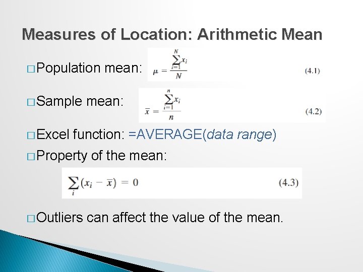
Measures of Location: Arithmetic Mean � Population � Sample � Excel mean: function: =AVERAGE(data range) � Property � Outliers of the mean: can affect the value of the mean.

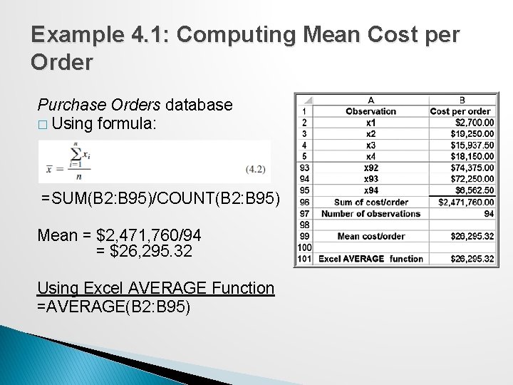
Example 4. 1: Computing Mean Cost per Order Purchase Orders database � Using formula: =SUM(B 2: B 95)/COUNT(B 2: B 95) Mean = $2, 471, 760/94 = $26, 295. 32 Using Excel AVERAGE Function =AVERAGE(B 2: B 95)

Measures of Location: Median The median specifies the middle value when the data are arranged from least to greatest. ◦ Half the data are below the median, and half the data are above it. ◦ For an odd number of observations, the median is the middle of the sorted numbers. ◦ For an even number of observations, the median is the mean of the two middle numbers. We could use the Sort option in Excel to rank-order the data and then determine the median. The Excel function =MEDIAN(data range) could also be used. The median is meaningful for ratio, interval, and ordinal data. Not affected by outliers.

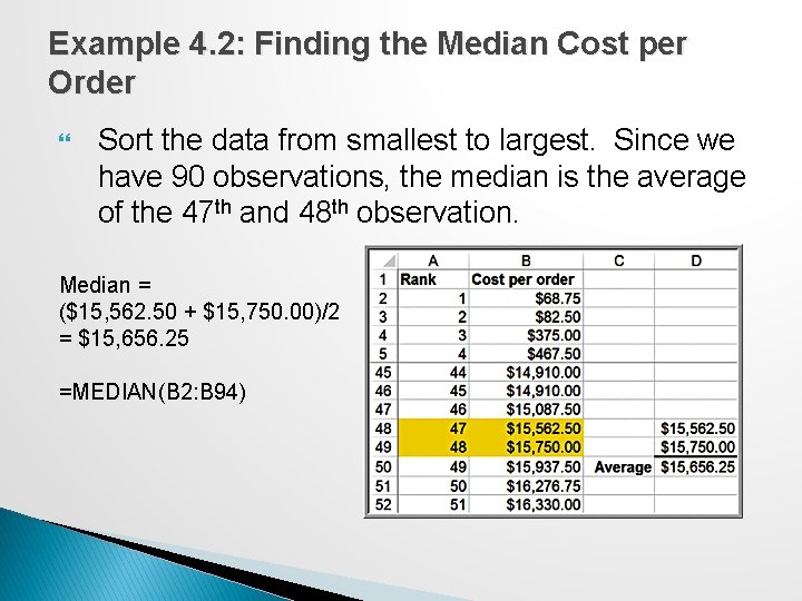
Example 4. 2: Finding the Median Cost per Order Sort the data from smallest to largest. Since we have 90 observations, the median is the average of the 47 th and 48 th observation. Median = ($15, 562. 50 + $15, 750. 00)/2 = $15, 656. 25 =MEDIAN(B 2: B 94)

Measures of Location: Mode The mode is the observation that occurs most frequently. The mode is most useful for data sets that contain a relatively small number of unique values. You can easily identify the mode from a frequency distribution by identifying the value or group having the largest frequency or from a histogram by identifying the highest bar. Excel function: =MODE. SNGL(data range). For multiple modes: =MODE. MULT(data range)

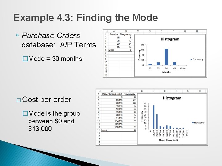
Example 4. 3: Finding the Mode Purchase Orders database: A/P Terms �Mode = 30 months � Cost per order �Mode is the group between $0 and $13, 000

Measures of Location: Midrange The midrange is the average of the greatest and least values in the data set. Caution must be exercised when using the midrange because extreme values easily distort the result. This is because the midrange uses only two pieces of data, whereas the mean uses all the data; thus, it is usually a much rougher estimate than the mean and is often used for only small sample sizes.

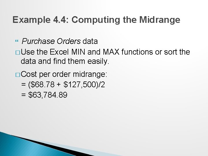
Example 4. 4: Computing the Midrange Purchase Orders data � Use the Excel MIN and MAX functions or sort the data and find them easily. � Cost per order midrange: = ($68. 78 + $127, 500)/2 = $63, 784. 89

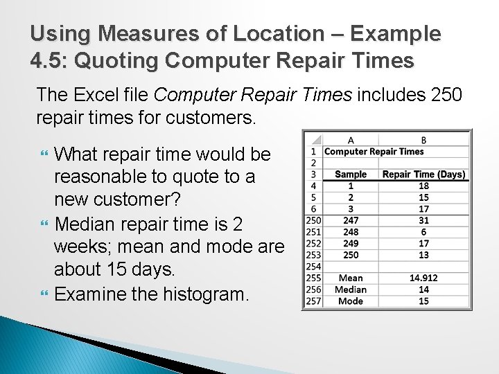
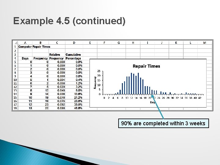
Using Measures of Location – Example 4. 5: Quoting Computer Repair Times The Excel file Computer Repair Times includes 250 repair times for customers. What repair time would be reasonable to quote to a new customer? Median repair time is 2 weeks; mean and mode are about 15 days. Examine the histogram.

Example 4. 5 (continued) 90% are completed within 3 weeks

Measures of Dispersion refers to the degree of variation in the data; that is, the numerical spread (or compactness) of the data. Key measures: ◦ ◦ Range Interquartile range Variance Standard deviation

Measures of Dispersion: Range The range is the simplest and is the difference between the maximum value and the minimum value in the data set. In Excel, compute as =MAX(data range) MIN(data range). The range is affected by outliers, and is often used only for very small data sets.

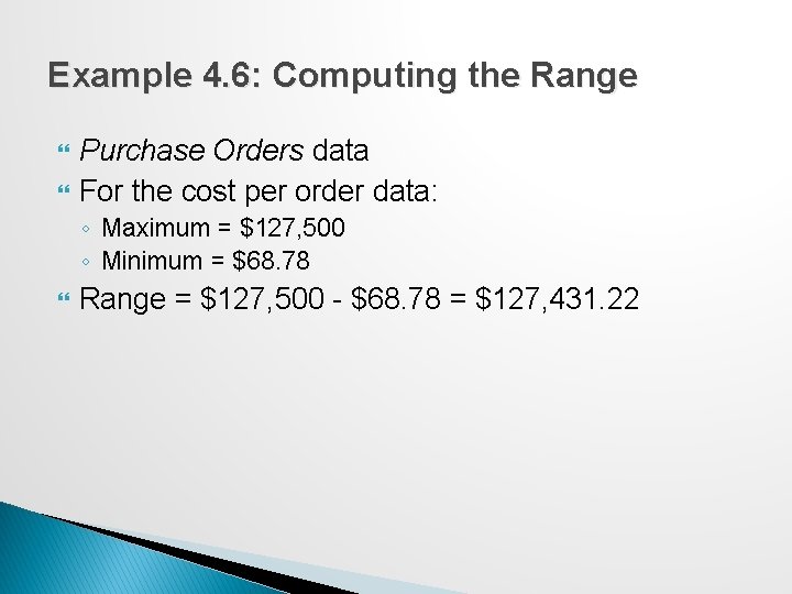
Example 4. 6: Computing the Range Purchase Orders data For the cost per order data: ◦ Maximum = $127, 500 ◦ Minimum = $68. 78 Range = $127, 500 - $68. 78 = $127, 431. 22

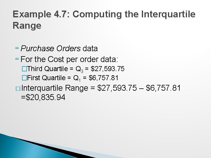
Measures of Dispersion: Interquartile Range The interquartile range (IQR), or the midspread is the difference between the first and third quartiles, Q 3 – Q 1. This includes only the middle 50% of the data and, therefore, is not influenced by extreme values.

Example 4. 7: Computing the Interquartile Range Purchase Orders data For the Cost per order data: �Third Quartile = Q 3 = $27, 593. 75 �First Quartile = Q 1 = $6, 757. 81 � Interquartile Range = $27, 593. 75 – $6, 757. 81 =$20, 835. 94

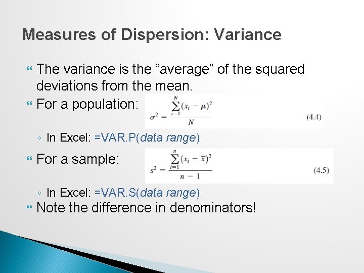
Measures of Dispersion: Variance The variance is the “average” of the squared deviations from the mean. For a population: ◦ In Excel: =VAR. P(data range) For a sample: ◦ In Excel: =VAR. S(data range) Note the difference in denominators!

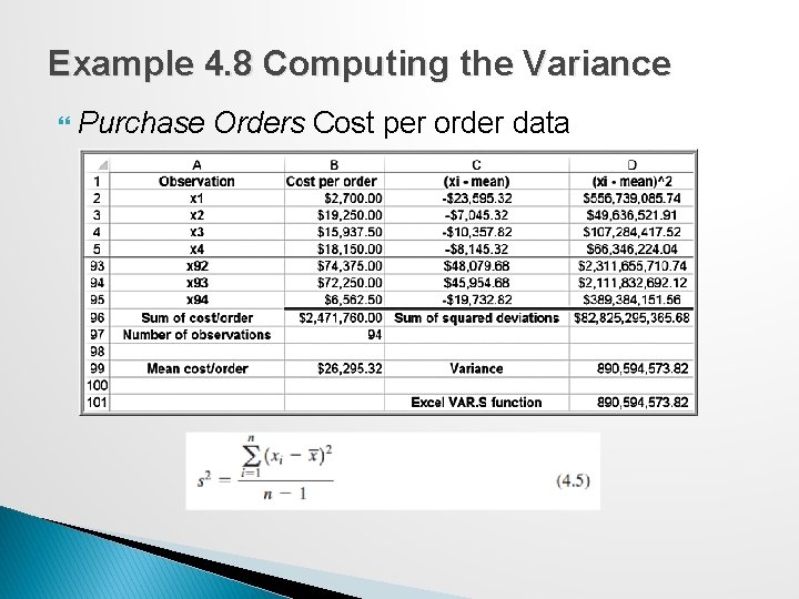
Example 4. 8 Computing the Variance Purchase Orders Cost per order data

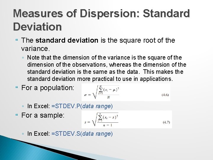
Measures of Dispersion: Standard Deviation The standard deviation is the square root of the variance. ◦ Note that the dimension of the variance is the square of the dimension of the observations, whereas the dimension of the standard deviation is the same as the data. This makes the standard deviation more practical to use in applications. For a population: ◦ In Excel: =STDEV. P(data range) For a sample: ◦ In Excel: =STDEV. S(data range)

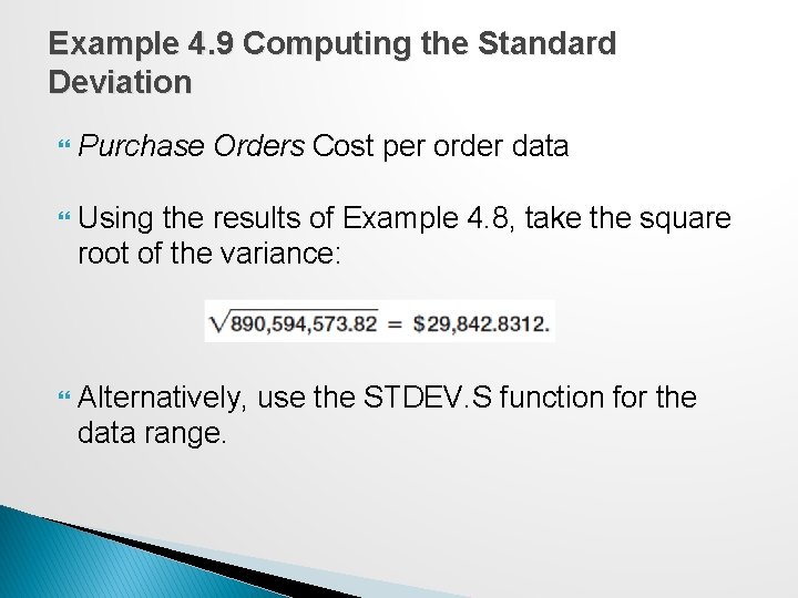
Example 4. 9 Computing the Standard Deviation Purchase Orders Cost per order data Using the results of Example 4. 8, take the square root of the variance: Alternatively, use the STDEV. S function for the data range.

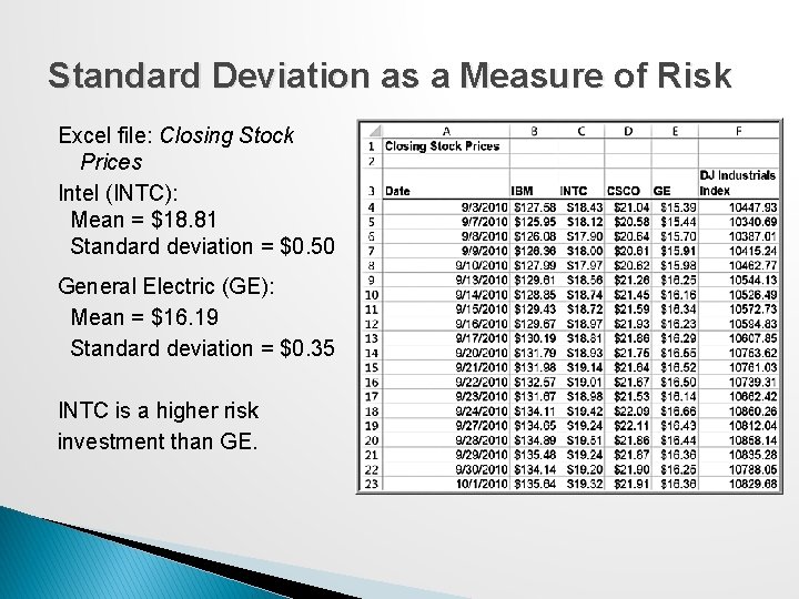
Standard Deviation as a Measure of Risk Excel file: Closing Stock Prices Intel (INTC): Mean = $18. 81 Standard deviation = $0. 50 General Electric (GE): Mean = $16. 19 Standard deviation = $0. 35 INTC is a higher risk investment than GE.

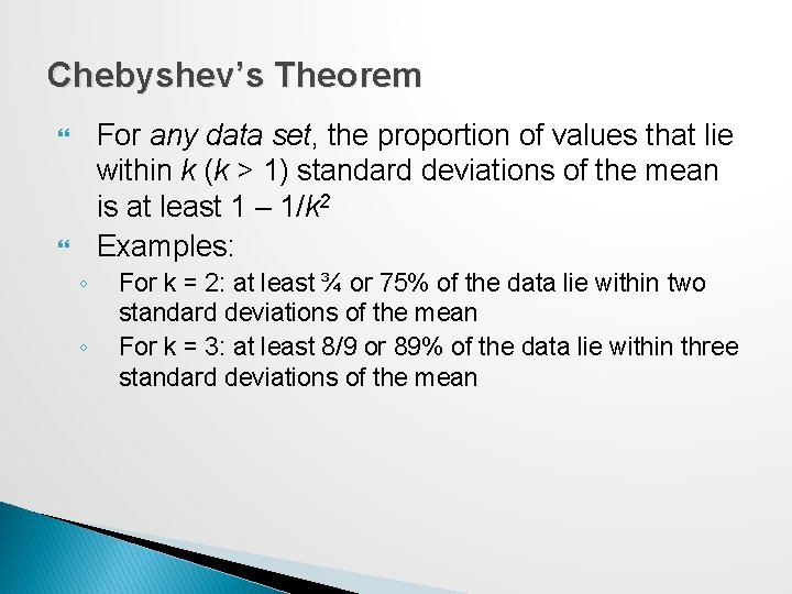
Chebyshev’s Theorem For any data set, the proportion of values that lie within k (k > 1) standard deviations of the mean is at least 1 – 1/k 2 Examples: ◦ ◦ For k = 2: at least ¾ or 75% of the data lie within two standard deviations of the mean For k = 3: at least 8/9 or 89% of the data lie within three standard deviations of the mean

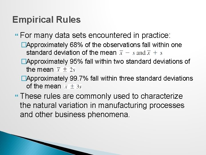
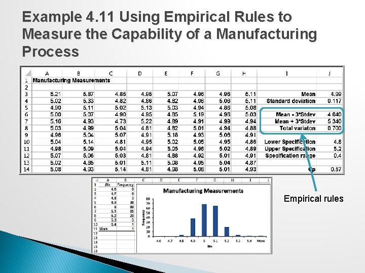
Empirical Rules For many data sets encountered in practice: �Approximately 68% of the observations fall within one standard deviation of the mean �Approximately 95% fall within two standard deviations of the mean �Approximately 99. 7% fall within three standard deviations of the mean These rules are commonly used to characterize the natural variation in manufacturing processes and other business phenomena.

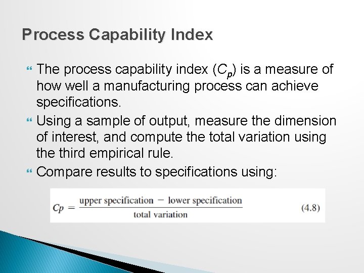
Process Capability Index The process capability index (Cp) is a measure of how well a manufacturing process can achieve specifications. Using a sample of output, measure the dimension of interest, and compute the total variation using the third empirical rule. Compare results to specifications using:

Example 4. 11 Using Empirical Rules to Measure the Capability of a Manufacturing Process Empirical rules

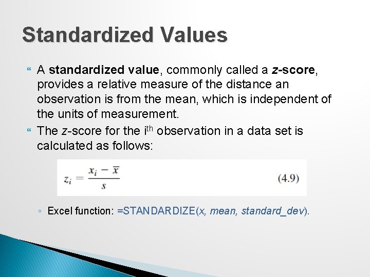
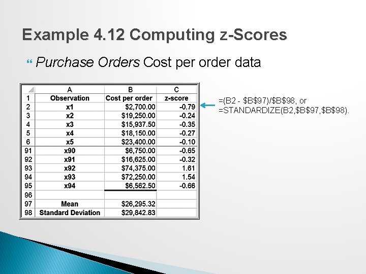
Standardized Values A standardized value, commonly called a z-score, provides a relative measure of the distance an observation is from the mean, which is independent of the units of measurement. The z-score for the ith observation in a data set is calculated as follows: ◦ Excel function: =STANDARDIZE(x, mean, standard_dev).

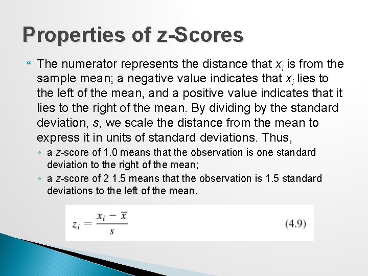
Properties of z-Scores The numerator represents the distance that xi is from the sample mean; a negative value indicates that xi lies to the left of the mean, and a positive value indicates that it lies to the right of the mean. By dividing by the standard deviation, s, we scale the distance from the mean to express it in units of standard deviations. Thus, ◦ a z-score of 1. 0 means that the observation is one standard deviation to the right of the mean; ◦ a z-score of 2 1. 5 means that the observation is 1. 5 standard deviations to the left of the mean.

Example 4. 12 Computing z-Scores Purchase Orders Cost per order data =(B 2 - $B$97)/$B$98, or =STANDARDIZE(B 2, $B$97, $B$98).

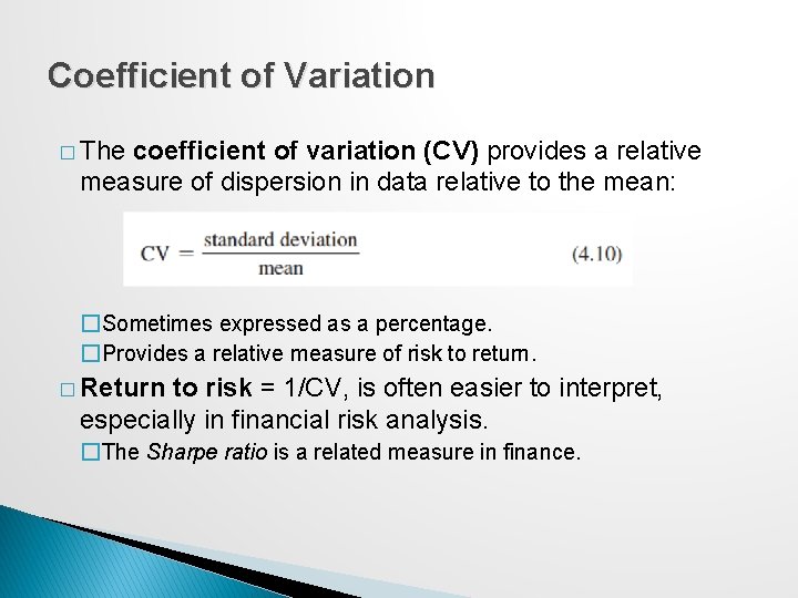
Coefficient of Variation � The coefficient of variation (CV) provides a relative measure of dispersion in data relative to the mean: �Sometimes expressed as a percentage. �Provides a relative measure of risk to return. � Return to risk = 1/CV, is often easier to interpret, especially in financial risk analysis. �The Sharpe ratio is a related measure in finance.

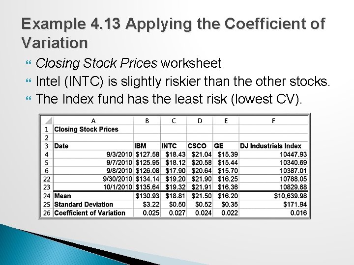
Example 4. 13 Applying the Coefficient of Variation Closing Stock Prices worksheet Intel (INTC) is slightly riskier than the other stocks. The Index fund has the least risk (lowest CV).

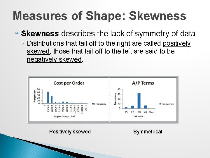
Measures of Shape: Skewness describes the lack of symmetry of data. ◦ Distributions that tail off to the right are called positively skewed; those that tail off to the left are said to be negatively skewed. Positively skewed Symmetrical

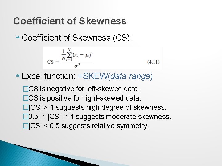
Coefficient of Skewness (CS): Excel function: =SKEW(data range) �CS is negative for left-skewed data. �CS is positive for right-skewed data. �|CS| > 1 suggests high degree of skewness. � 0. 5 ≤ |CS| ≤ 1 suggests moderate skewness. �|CS| < 0. 5 suggests relative symmetry.

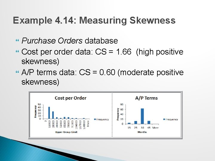
Example 4. 14: Measuring Skewness Purchase Orders database Cost per order data: CS = 1. 66 (high positive skewness) A/P terms data: CS = 0. 60 (moderate positive skewness)

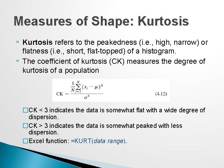
Measures of Shape: Kurtosis refers to the peakedness (i. e. , high, narrow) or flatness (i. e. , short, flat-topped) of a histogram. The coefficient of kurtosis (CK) measures the degree of kurtosis of a population �CK < 3 indicates the data is somewhat flat with a wide degree of dispersion. �CK > 3 indicates the data is somewhat peaked with less dispersion. �Excel function: =KURT(data range).

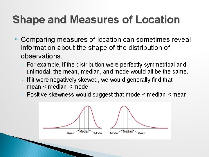
Shape and Measures of Location Comparing measures of location can sometimes reveal information about the shape of the distribution of observations. ◦ For example, if the distribution were perfectly symmetrical and unimodal, the mean, median, and mode would all be the same. ◦ If it were negatively skewed, we would generally find that mean < median < mode ◦ Positive skewness would suggest that mode < median < mean

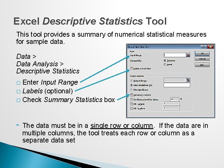
Excel Descriptive Statistics Tool This tool provides a summary of numerical statistical measures for sample data. Data > Data Analysis > Descriptive Statistics Enter Input Range � Labels (optional) � Check Summary Statistics box � The data must be in a single row or column. If the data are in multiple columns, the tool treats each row or column as a separate data set

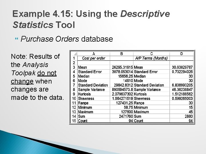
Example 4. 15: Using the Descriptive Statistics Tool Purchase Orders database Note: Results of the Analysis Toolpak do not change when changes are made to the data.

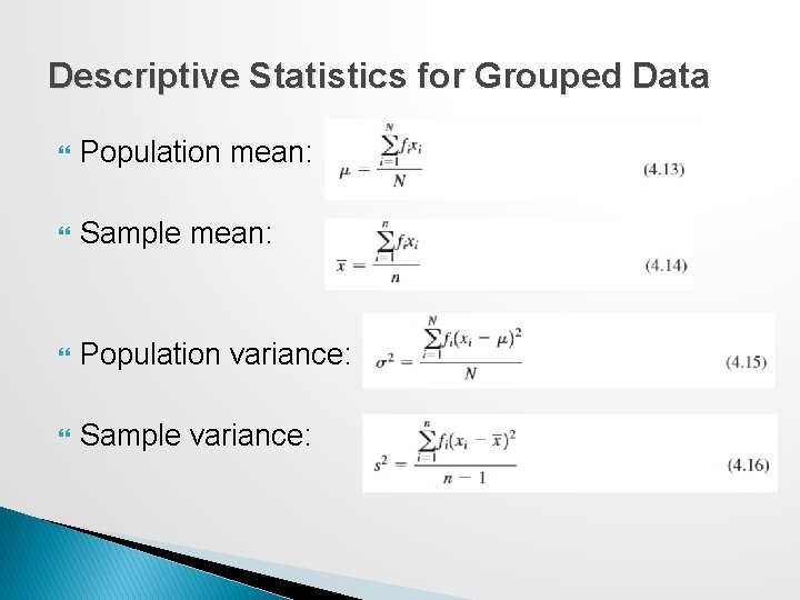
Descriptive Statistics for Grouped Data Population mean: Sample mean: Population variance: Sample variance:

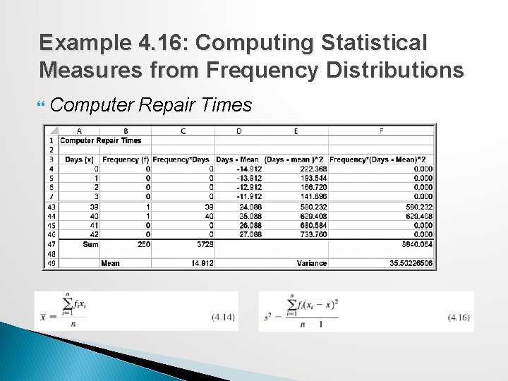
Example 4. 16: Computing Statistical Measures from Frequency Distributions Computer Repair Times

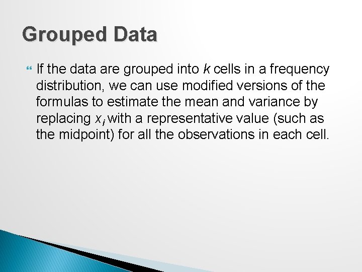
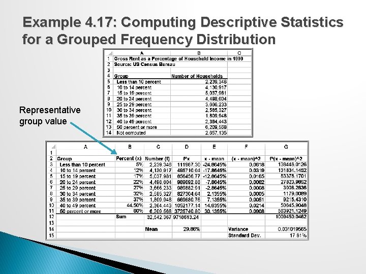
Grouped Data If the data are grouped into k cells in a frequency distribution, we can use modified versions of the formulas to estimate the mean and variance by replacing xi with a representative value (such as the midpoint) for all the observations in each cell.

Example 4. 17: Computing Descriptive Statistics for a Grouped Frequency Distribution Representative group value

Descriptive Statistics for Categorical Data: The Proportion The proportion, denoted by p, is the fraction of data that have a certain characteristic. Proportions are key descriptive statistics for categorical data, such as defects or errors in quality control applications or consumer preferences in market research.

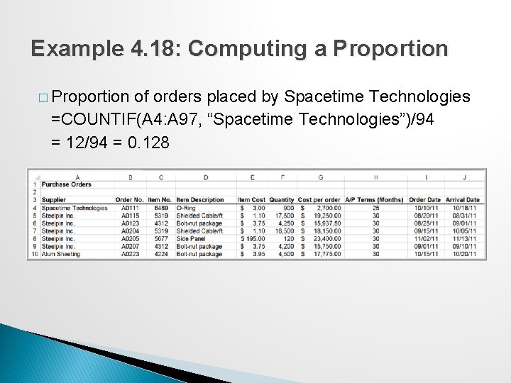
Example 4. 18: Computing a Proportion � Proportion of orders placed by Spacetime Technologies =COUNTIF(A 4: A 97, “Spacetime Technologies”)/94 = 12/94 = 0. 128

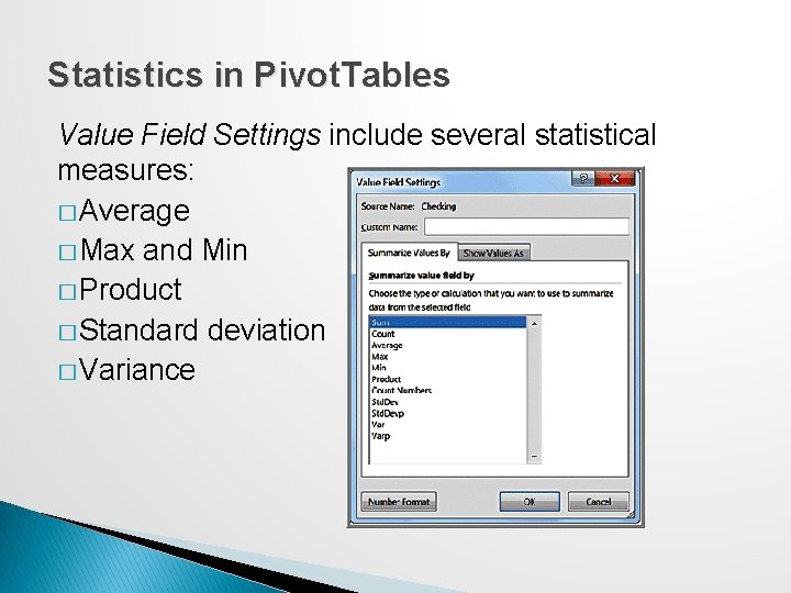
Statistics in Pivot. Tables Value Field Settings include several statistical measures: � Average � Max and Min � Product � Standard deviation � Variance

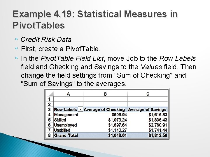
Example 4. 19: Statistical Measures in Pivot. Tables Credit Risk Data First, create a Pivot. Table. In the Pivot. Table Field List, move Job to the Row Labels field and Checking and Savings to the Values field. Then change the field settings from “Sum of Checking” and “Sum of Savings” to the averages.

Measures of Association Two variables have a strong statistical relationship with one another if they appear to move together. When two variables appear to be related, you might suspect a cause-and-effect relationship. Sometimes, however, statistical relationships exist even though a change in one variable is not caused by a change in the other.

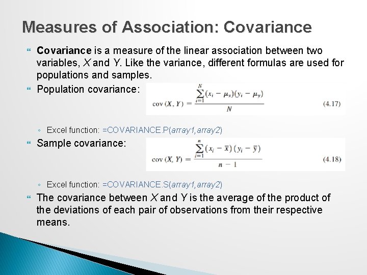
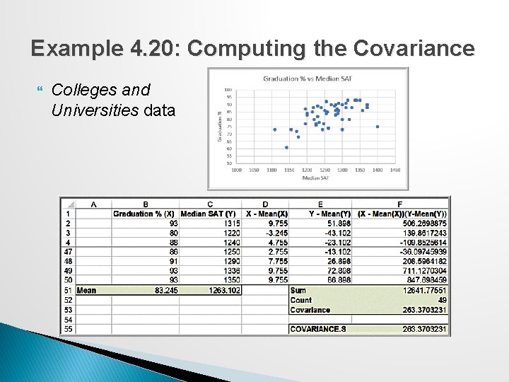
Measures of Association: Covariance is a measure of the linear association between two variables, X and Y. Like the variance, different formulas are used for populations and samples. Population covariance: ◦ Excel function: =COVARIANCE. P(array 1, array 2) Sample covariance: ◦ Excel function: =COVARIANCE. S(array 1, array 2) The covariance between X and Y is the average of the product of the deviations of each pair of observations from their respective means.

Example 4. 20: Computing the Covariance Colleges and Universities data

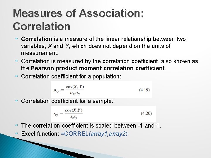
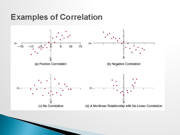
Measures of Association: Correlation is a measure of the linear relationship between two variables, X and Y, which does not depend on the units of measurement. Correlation is measured by the correlation coefficient, also known as the Pearson product moment correlation coefficient. Correlation coefficient for a population: Correlation coefficient for a sample: The correlation coefficient is scaled between -1 and 1. Excel function: =CORREL(array 1, array 2)

Examples of Correlation

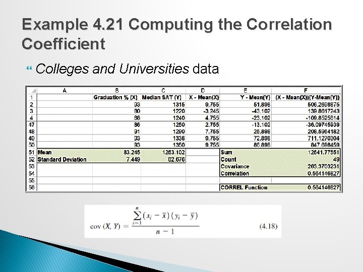
Example 4. 21 Computing the Correlation Coefficient Colleges and Universities data

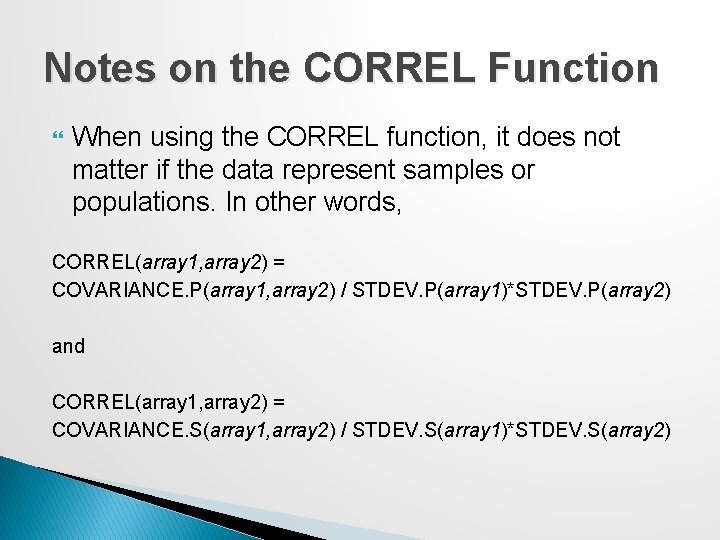
Notes on the CORREL Function When using the CORREL function, it does not matter if the data represent samples or populations. In other words, CORREL(array 1, array 2) = COVARIANCE. P(array 1, array 2) / STDEV. P(array 1)*STDEV. P(array 2) and CORREL(array 1, array 2) = COVARIANCE. S(array 1, array 2) / STDEV. S(array 1)*STDEV. S(array 2)

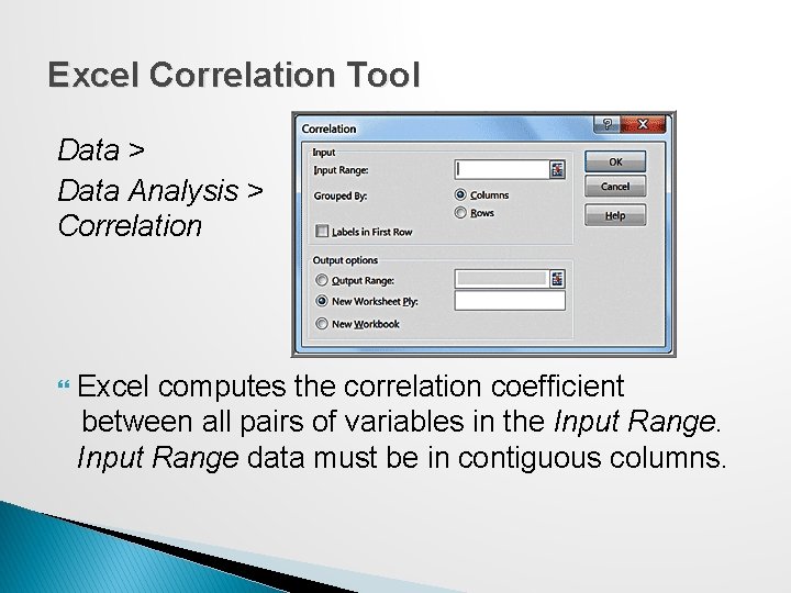
Excel Correlation Tool Data > Data Analysis > Correlation Excel computes the correlation coefficient between all pairs of variables in the Input Range data must be in contiguous columns.

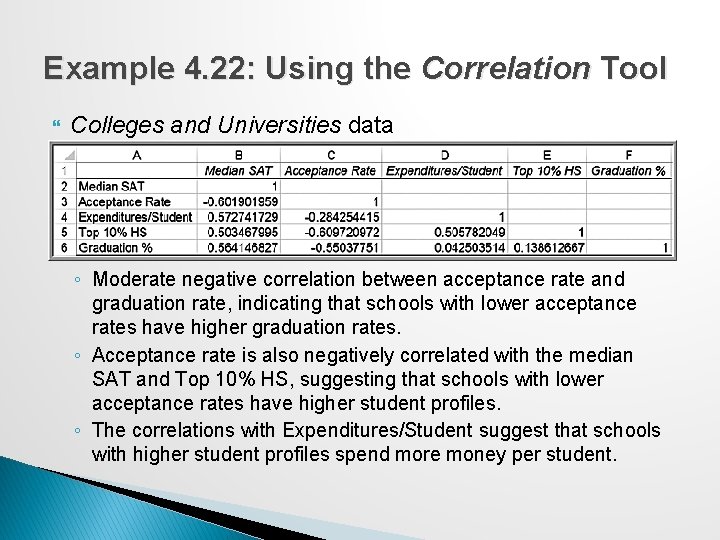
Example 4. 22: Using the Correlation Tool Colleges and Universities data ◦ Moderate negative correlation between acceptance rate and graduation rate, indicating that schools with lower acceptance rates have higher graduation rates. ◦ Acceptance rate is also negatively correlated with the median SAT and Top 10% HS, suggesting that schools with lower acceptance rates have higher student profiles. ◦ The correlations with Expenditures/Student suggest that schools with higher student profiles spend more money per student.

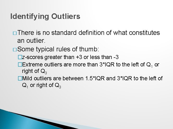
Identifying Outliers � There is no standard definition of what constitutes an outlier. � Some typical rules of thumb: �z-scores greater than +3 or less than -3 �Extreme outliers are more than 3*IQR to the left of Q 1 or right of Q 3 �Mild outliers are between 1. 5*IQR and 3*IQR to the left of Q 1 or right of Q 3

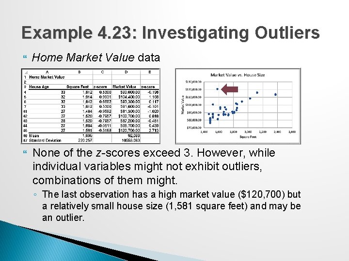
Example 4. 23: Investigating Outliers Home Market Value data None of the z-scores exceed 3. However, while individual variables might not exhibit outliers, combinations of them might. ◦ The last observation has a high market value ($120, 700) but a relatively small house size (1, 581 square feet) and may be an outlier.

Statistical Thinking in Business Decisions Statistical Thinking is a philosophy of learning and action for improvement, based on principles that: �all work occurs in a system of interconnected processes �variation exists in all processes �better performance results from understanding and reducing variation Work gets done in any organization through processes — systematic ways of doing things that achieve desired results. Understanding business processes provides the context for determining the effects of variation and the proper type of action to be taken.

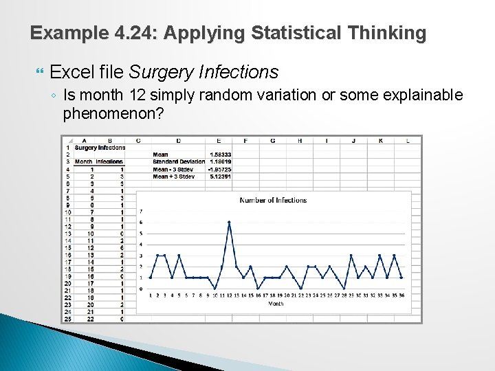
Example 4. 24: Applying Statistical Thinking Excel file Surgery Infections ◦ Is month 12 simply random variation or some explainable phenomenon?

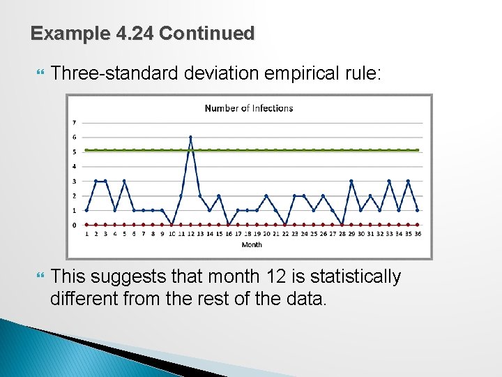
Example 4. 24 Continued Three-standard deviation empirical rule: This suggests that month 12 is statistically different from the rest of the data.

Variability in Samples Different samples from any population will vary. ◦ They will have different means, standard deviations, and other statistical measures ◦ They will have differences in the shapes of histograms. Samples are extremely sensitive to the sample size – the number of observations included in the samples.

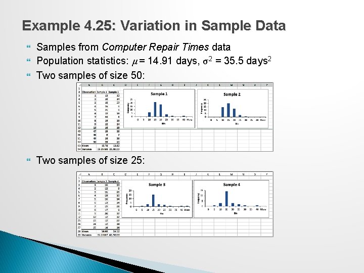
Example 4. 25: Variation in Sample Data Samples from Computer Repair Times data Population statistics: μ = 14. 91 days, σ2 = 35. 5 days 2 Two samples of size 50: Two samples of size 25: