Chapter 4 Describing the Relation Between Two Variables

Chapter 4 Describing the Relation Between Two Variables Sullivan – Statistics: Informed Decisions Using Data – 2 nd Edition – Chapter 4 Introduction – Slide 1 of 3

Overview ● Data for a single variable is univariate data ● Many or most real world models have more than one variable … multivariate data ● In this chapter we will study the relations between two variables … bivariate data Sullivan – Statistics: Informed Decisions Using Data – 2 nd Edition – Chapter 4 Introduction – Slide 2 of 3

Chapter 4 ● Chapter 4 – Describing the Relation Between Two Variables Only section 1 and 2 § § Scatter Diagrams and Correlation Least-Squares Regression Sullivan – Statistics: Informed Decisions Using Data – 2 nd Edition – Chapter 4 Introduction – Slide 3 of 3

Chapter 4 Section 1 Scatter Diagrams and Correlation Sullivan – Statistics: Informed Decisions Using Data – 2 nd Edition – Chapter 4 Introduction – Slide 4 of 3

Chapter 4 – Section 1 ● In many studies, we measure more than one variable for each individual ● Some examples are § Rainfall amounts and plant growth § Exercise and cholesterol levels for a group of people § Height and weight for a group of people ● In these cases, we are interested in whether the two variables have some kind of a relationship Sullivan – Statistics: Informed Decisions Using Data – 2 nd Edition – Chapter 4 Introduction – Slide 5 of 3

Chapter 4 – Section 1 ● When we have two variables, they could be related in one of several different ways § They could be unrelated § One variable (the explanatory or predictor variable) could be used to explain the other (the response or dependent variable) § One variable could be thought of as causing the other variable to change ● In this chapter, we examine the second case … explanatory and response variables Sullivan – Statistics: Informed Decisions Using Data – 2 nd Edition – Chapter 4 Introduction – Slide 6 of 3

Chapter 4 – Section 1 ● Sometimes it is not clear which variable is the explanatory variable and which is the response variable ● Sometimes the two variables are related without either one being an explanatory variable ● Sometimes the two variables are both affected by a third variable, a lurking variable, that had not been included in the study Sullivan – Statistics: Informed Decisions Using Data – 2 nd Edition – Chapter 4 Introduction – Slide 7 of 3

Chapter 4 – Section 1 ● An example of a lurking variable ● A researcher studies a group of elementary school children § Y = the student’s height § X = the student’s shoe size ● It is not reasonable to claim that shoe size causes height to change ● The lurking variable of age affects both of these two variables Sullivan – Statistics: Informed Decisions Using Data – 2 nd Edition – Chapter 4 Introduction – Slide 8 of 3

Chapter 4 – Section 1 ● Some other examples ● Rainfall amounts and plant growth § Explanatory variable – rainfall § Response variable – plant growth § Possible lurking variable – amount of sunlight ● Exercise and cholesterol levels § Explanatory variable – amount of exercise § Response variable – cholesterol level § Possible lurking variable – diet Sullivan – Statistics: Informed Decisions Using Data – 2 nd Edition – Chapter 4 Introduction – Slide 9 of 3

Chapter 4 – Section 1 ● The most useful graph to show the relationship between two quantitative variables is the scatter diagram ● Each individual is represented by a point in the diagram § The explanatory (X) variable is plotted on the horizontal scale § The response (Y) variable is plotted on the vertical scale Sullivan – Statistics: Informed Decisions Using Data – 2 nd Edition – Chapter 4 Introduction – Slide 10 of 3

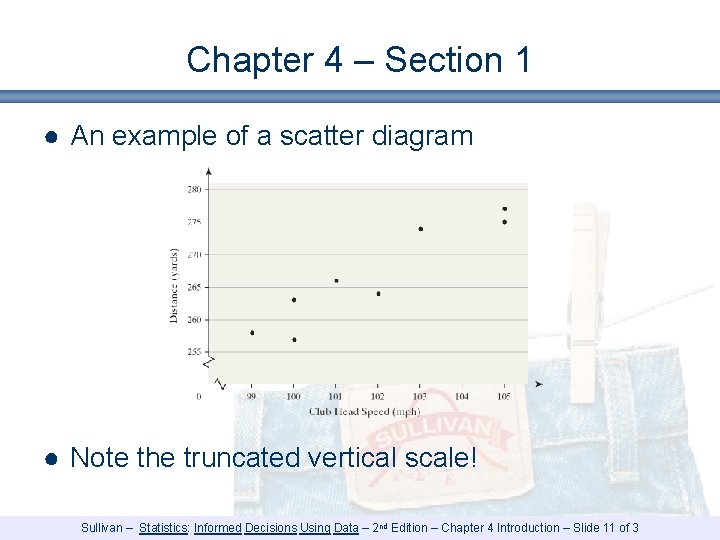
Chapter 4 – Section 1 ● An example of a scatter diagram ● Note the truncated vertical scale! Sullivan – Statistics: Informed Decisions Using Data – 2 nd Edition – Chapter 4 Introduction – Slide 11 of 3

Chapter 4 – Section 1 ● There are several different types of relations between two variables § A relationship is linear when, plotted on a scatter diagram, the points follow the general pattern of a line § A relationship is nonlinear when, plotted on a scatter diagram, the points follow a general pattern, but it is not a line § A relationship has no correlation when, plotted on a scatter diagram, the points do not show any pattern Sullivan – Statistics: Informed Decisions Using Data – 2 nd Edition – Chapter 4 Introduction – Slide 12 of 3

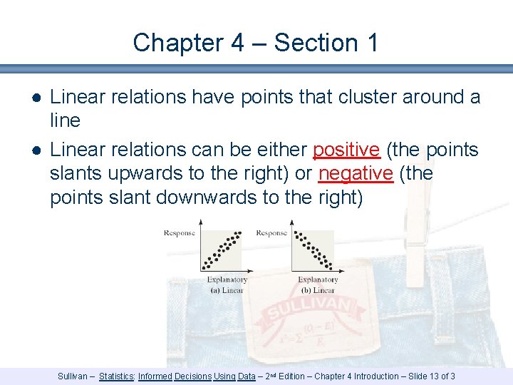
Chapter 4 – Section 1 ● Linear relations have points that cluster around a line ● Linear relations can be either positive (the points slants upwards to the right) or negative (the points slant downwards to the right) Sullivan – Statistics: Informed Decisions Using Data – 2 nd Edition – Chapter 4 Introduction – Slide 13 of 3

Chapter 4 – Section 1 ● For positive (linear) associations § Above average values of one variable are associated with above average values of the other (above/above, the points trend right and upwards) § Below average values of one variable are associated with below average values of the other (below/below, the points trend left and downwards) ● Examples § “Age” and “Height” for children § “Temperature” and “Sales of ice cream” Sullivan – Statistics: Informed Decisions Using Data – 2 nd Edition – Chapter 4 Introduction – Slide 14 of 3

Chapter 4 – Section 1 ● For negative (linear) associations § Above average values of one variable are associated with below average values of the other (above/below, the points trend right and downwards) § Below average values of one variable are associated with above average values of the other (below/above, the points trend left and upwards) ● Examples § “Age” and “Time required to run 50 meters” for children § “Temperature” and “Sales of hot chocolate” Sullivan – Statistics: Informed Decisions Using Data – 2 nd Edition – Chapter 4 Introduction – Slide 15 of 3

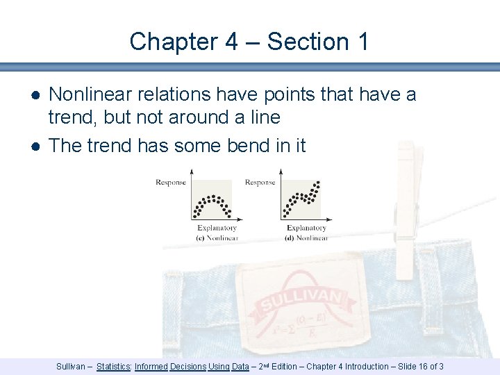
Chapter 4 – Section 1 ● Nonlinear relations have points that have a trend, but not around a line ● The trend has some bend in it Sullivan – Statistics: Informed Decisions Using Data – 2 nd Edition – Chapter 4 Introduction – Slide 16 of 3

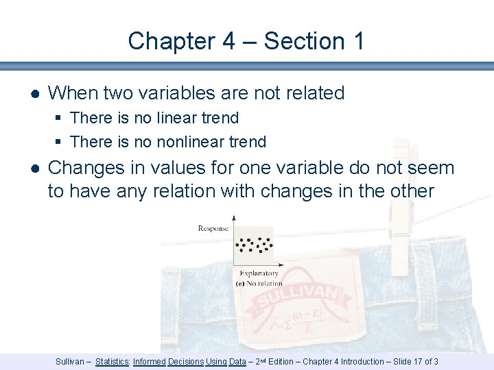
Chapter 4 – Section 1 ● When two variables are not related § There is no linear trend § There is no nonlinear trend ● Changes in values for one variable do not seem to have any relation with changes in the other Sullivan – Statistics: Informed Decisions Using Data – 2 nd Edition – Chapter 4 Introduction – Slide 17 of 3

Chapter 4 – Section 1 ● Nonlinear relations and no relations are very different § Nonlinear relations are definitely patterns … just not patterns that look like lines § No relations are when no patterns appear at all Sullivan – Statistics: Informed Decisions Using Data – 2 nd Edition – Chapter 4 Introduction – Slide 18 of 3

Chapter 4 – Section 1 ● Examples of nonlinear relations § “Age” and “Height” for people (including both children and adults) § “Temperature” and “Comfort level” for people ● Examples of no relations § “Temperature” and “Closing price of the Dow Jones Industrials Index” (probably) § “Age” and “Last digit of telephone number” for adults Sullivan – Statistics: Informed Decisions Using Data – 2 nd Edition – Chapter 4 Introduction – Slide 19 of 3

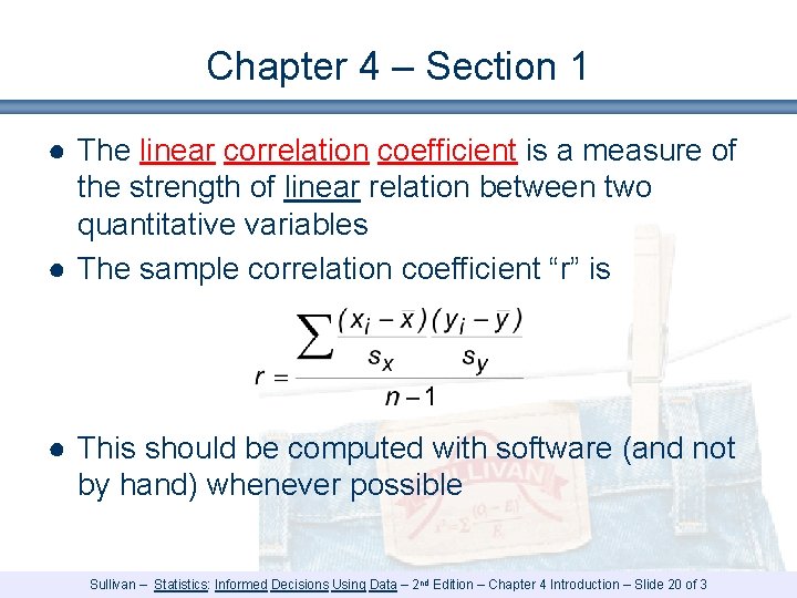
Chapter 4 – Section 1 ● The linear correlation coefficient is a measure of the strength of linear relation between two quantitative variables ● The sample correlation coefficient “r” is ● This should be computed with software (and not by hand) whenever possible Sullivan – Statistics: Informed Decisions Using Data – 2 nd Edition – Chapter 4 Introduction – Slide 20 of 3

Chapter 4 – Section 1 ● Some properties of the linear correlation coefficient § r is a unitless measure (so that r would be the same for a data set whether x and y are measured in feet, inches, meters, or fathoms) § r is always between – 1 and +1 § Positive values of r correspond to positive relations § Negative values of r correspond to negative relations Sullivan – Statistics: Informed Decisions Using Data – 2 nd Edition – Chapter 4 Introduction – Slide 21 of 3

Chapter 4 – Section 1 ● Some more properties of the linear correlation coefficient § The closer r is to +1, the stronger the positive relation … when r = +1, there is a perfect positive relation § The closer r is to – 1, the stronger the negative relation … when r = – 1, there is a perfect negative relation § The closer r is to 0, the less of a linear relation (either positive or negative) Sullivan – Statistics: Informed Decisions Using Data – 2 nd Edition – Chapter 4 Introduction – Slide 22 of 3

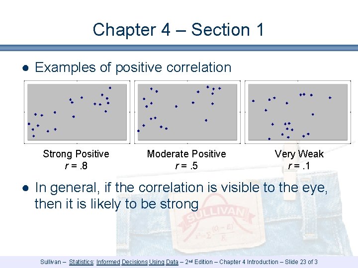
Chapter 4 – Section 1 ● Examples of positive correlation Strong Positive r =. 8 Moderate Positive r =. 5 Very Weak r =. 1 ● In general, if the correlation is visible to the eye, then it is likely to be strong Sullivan – Statistics: Informed Decisions Using Data – 2 nd Edition – Chapter 4 Introduction – Slide 23 of 3

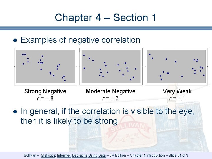
Chapter 4 – Section 1 ● Examples of negative correlation Strong Negative r = –. 8 Moderate Negative r = –. 5 Very Weak r = –. 1 ● In general, if the correlation is visible to the eye, then it is likely to be strong Sullivan – Statistics: Informed Decisions Using Data – 2 nd Edition – Chapter 4 Introduction – Slide 24 of 3

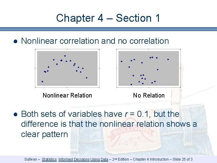
Chapter 4 – Section 1 ● Nonlinear correlation and no correlation Nonlinear Relation No Relation ● Both sets of variables have r = 0. 1, but the difference is that the nonlinear relation shows a clear pattern Sullivan – Statistics: Informed Decisions Using Data – 2 nd Edition – Chapter 4 Introduction – Slide 25 of 3

Chapter 4 – Section 1 ● Correlation is not causation! ● Just because two variables are correlated does not mean that one causes the other to change ● There is a strong correlation between shoe sizes and vocabulary sizes for grade school children § Clearly larger shoe sizes do not cause larger vocabularies § Clearly larger vocabularies do not cause larger shoe sizes ● Often lurking variables result in confounding Sullivan – Statistics: Informed Decisions Using Data – 2 nd Edition – Chapter 4 Introduction – Slide 26 of 3

Summary: Chapter 4 – Section 1 ● Correlation between two variables can be described with both visual (graphic) and numeric methods ● Visual methods § Scatter diagrams ● Numeric methods § Linear correlation coefficient Sullivan – Statistics: Informed Decisions Using Data – 2 nd Edition – Chapter 4 Introduction – Slide 27 of 3

Chapter 4 Section 2 Least-Squares Regression Sullivan – Statistics: Informed Decisions Using Data – 2 nd Edition – Chapter 4 Introduction – Slide 28 of 3

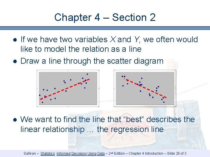
Chapter 4 – Section 2 ● If we have two variables X and Y, we often would like to model the relation as a line ● Draw a line through the scatter diagram ● We want to find the line that “best” describes the linear relationship … the regression line Sullivan – Statistics: Informed Decisions Using Data – 2 nd Edition – Chapter 4 Introduction – Slide 29 of 3

Chapter 4 – Section 2 ● We want to use a linear model ● Linear models can be written in several different (equivalent) ways § y=mx+b § y – y 1 = m (x – x 1) § y = b 1 x + b 0 ● Because the slope and the intercept are important to analyze, we will use y = b 1 x + b 0 Sullivan – Statistics: Informed Decisions Using Data – 2 nd Edition – Chapter 4 Introduction – Slide 30 of 3

Chapter 4 – Section 2 ● The difference between the observed value and the predicted value is called an error or residual ● The formula for the residual is always Residual = Observed – Predicted Sullivan – Statistics: Informed Decisions Using Data – 2 nd Edition – Chapter 4 Introduction – Slide 31 of 3

Chapter 4 – Section 2 ● For example, say that we want to predict a value of y for a specific value of x § Assume that we are using y = 10 x + 25 as our model § To predict the value of y when x = 3, the model gives us y = 10 3 + 25 = 55, or a predicted value of 55 § Assume the actual value of y for x = 3 is equal to 50 § The actual value is 50, the predicted value is 55, so the residual (or error) is 50 – 55 = – 5 Sullivan – Statistics: Informed Decisions Using Data – 2 nd Edition – Chapter 4 Introduction – Slide 32 of 3

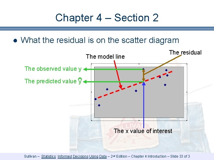
Chapter 4 – Section 2 ● What the residual is on the scatter diagram The model line The residual The observed value y The predicted value y The x value of interest Sullivan – Statistics: Informed Decisions Using Data – 2 nd Edition – Chapter 4 Introduction – Slide 33 of 3

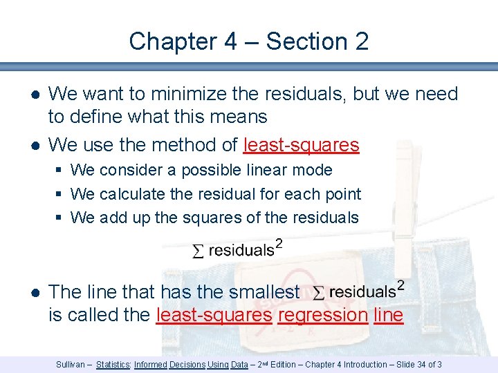
Chapter 4 – Section 2 ● We want to minimize the residuals, but we need to define what this means ● We use the method of least-squares § We consider a possible linear mode § We calculate the residual for each point § We add up the squares of the residuals ● The line that has the smallest is called the least-squares regression line Sullivan – Statistics: Informed Decisions Using Data – 2 nd Edition – Chapter 4 Introduction – Slide 34 of 3

Chapter 4 – Section 2 ● The equation for the least-squares regression line is given by y = b 1 x + b 0 § b 1 is the slope of the least-squares regression line § b 0 is the y-intercept of the least-squares regression line Sullivan – Statistics: Informed Decisions Using Data – 2 nd Edition – Chapter 4 Introduction – Slide 35 of 3

Chapter 4 – Section 2 ● Finding the values of b 1 and b 0, by hand, is a very tedious process ● You should use software for this ● Finding the coefficients b 1 and b 0 is only the first step of a regression analysis § We need to interpret the slope b 1 § We need to interpret the y-intercept b 0 Sullivan – Statistics: Informed Decisions Using Data – 2 nd Edition – Chapter 4 Introduction – Slide 36 of 3

Chapter 4 – Section 2 ● Interpreting the slope b 1 § The slope is sometimes referred to as § The slope is also sometimes referred to as ● The slope relates changes in y to changes in x Sullivan – Statistics: Informed Decisions Using Data – 2 nd Edition – Chapter 4 Introduction – Slide 37 of 3

Chapter 4 – Section 2 ● For example, if b 1 = 4 § If x increases by 1, then y will increase by 4 § If x decreases by 1, then y will decrease by 4 § A positive linear relationship ● For example, if b 1 = – 7 § If x increases by 1, then y will decrease by 7 § If x decreases by 1, then y will increase by 7 § A negative linear relationship Sullivan – Statistics: Informed Decisions Using Data – 2 nd Edition – Chapter 4 Introduction – Slide 38 of 3

Chapter 4 – Section 2 ● For example, say that a researcher studies the population in a town (the y or response variable) in each year (the x or predictor variable) § To simplify the calculations, years are measured from 1900 (i. e. x = 55 is the year 1955) ● The model used is y = 300 x + 12, 000 ● A slope of 300 means that the model predicts that, on the average, the population increases by 300 per year Sullivan – Statistics: Informed Decisions Using Data – 2 nd Edition – Chapter 4 Introduction – Slide 39 of 3

Chapter 4 – Section 2 ● Interpreting the y-intercept b 0 ● Sometimes b 0 has an interpretation, and sometimes not § If 0 is a reasonable value for x, then b 0 can be interpreted as the value of y when x is 0 § If 0 is not a reasonable value for x, then b 0 does not have an interpretation ● In general, we should not use the model for values of x that are much larger or much smaller than the observed values Sullivan – Statistics: Informed Decisions Using Data – 2 nd Edition – Chapter 4 Introduction – Slide 40 of 3

Chapter 4 – Section 2 ● For example, say that a researcher studies the population in a town (the y or response variable) in each year (the x or predictor variable) § To simplify the calculations, years are measured from 1900 (i. e. x = 55 is the year 1955) ● The model used is y = 300 x + 12, 000 ● An intercept of 12, 000 means that the model predicts that the town had a population of 12, 000 in the year 1900 (i. e. when x = 0) Sullivan – Statistics: Informed Decisions Using Data – 2 nd Edition – Chapter 4 Introduction – Slide 41 of 3

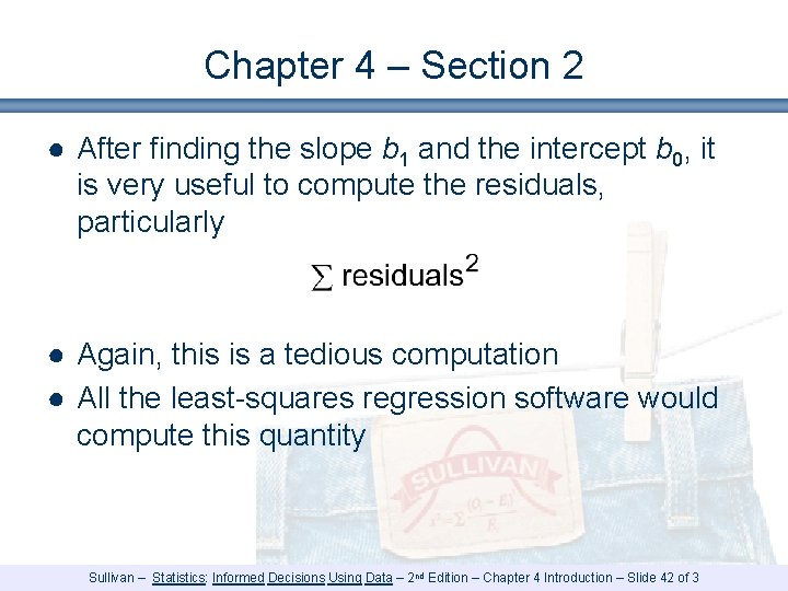
Chapter 4 – Section 2 ● After finding the slope b 1 and the intercept b 0, it is very useful to compute the residuals, particularly ● Again, this is a tedious computation ● All the least-squares regression software would compute this quantity Sullivan – Statistics: Informed Decisions Using Data – 2 nd Edition – Chapter 4 Introduction – Slide 42 of 3

Summary: Chapter 4 – Section 2 ● We can find the least-squares regression line that is the “best” linear model for a set of data ● The slope can be interpreted as the change in y for every change of 1 in x ● The intercept can be interpreted as the value of y when x is 0, as long as a value of 0 for x is reasonable Sullivan – Statistics: Informed Decisions Using Data – 2 nd Edition – Chapter 4 Introduction – Slide 43 of 3