Chapter 4 Continuous Random Variables Continuous Probability Distributions

Chapter 4 Continuous Random Variables

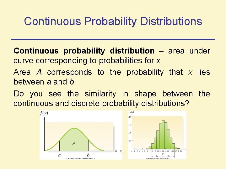
Continuous Probability Distributions Continuous probability distribution – area under curve corresponding to probabilities for x Area A corresponds to the probability that x lies between a and b Do you see the similarity in shape between the continuous and discrete probability distributions?

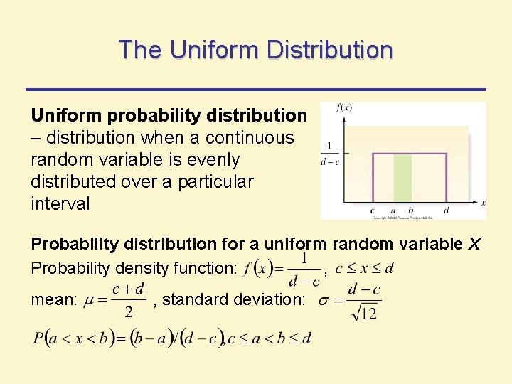
The Uniform Distribution Uniform probability distribution – distribution when a continuous random variable is evenly distributed over a particular interval Probability distribution for a uniform random variable X Probability density function: , mean: , standard deviation:

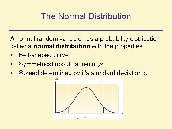
The Normal Distribution A normal random variable has a probability distribution called a normal distribution with the properties: • Bell-shaped curve • Symmetrical about its mean μ • Spread determined by it’s standard deviation σ

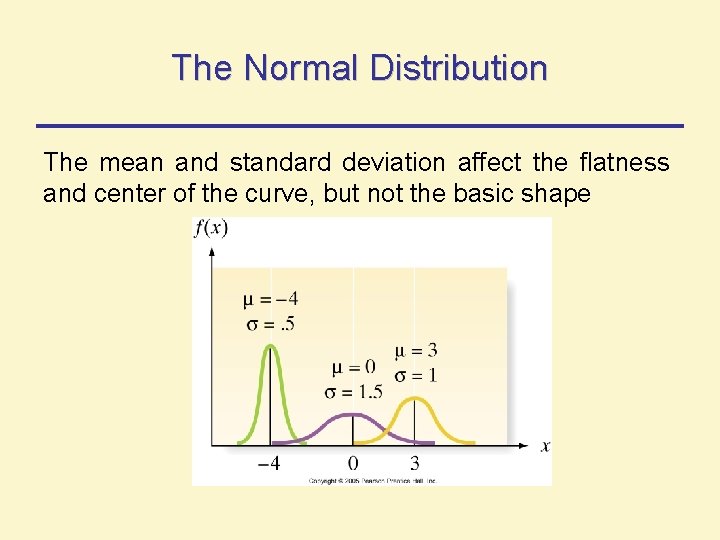
The Normal Distribution The mean and standard deviation affect the flatness and center of the curve, but not the basic shape

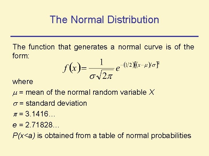
The Normal Distribution The function that generates a normal curve is of the form: where = mean of the normal random variable X = standard deviation = 3. 1416… e = 2. 71828… P(x<a) is obtained from a table of normal probabilities

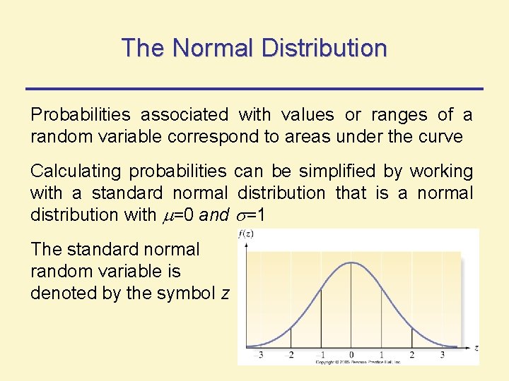
The Normal Distribution Probabilities associated with values or ranges of a random variable correspond to areas under the curve Calculating probabilities can be simplified by working with a standard normal distribution that is a normal distribution with =0 and =1 The standard normal random variable is denoted by the symbol z

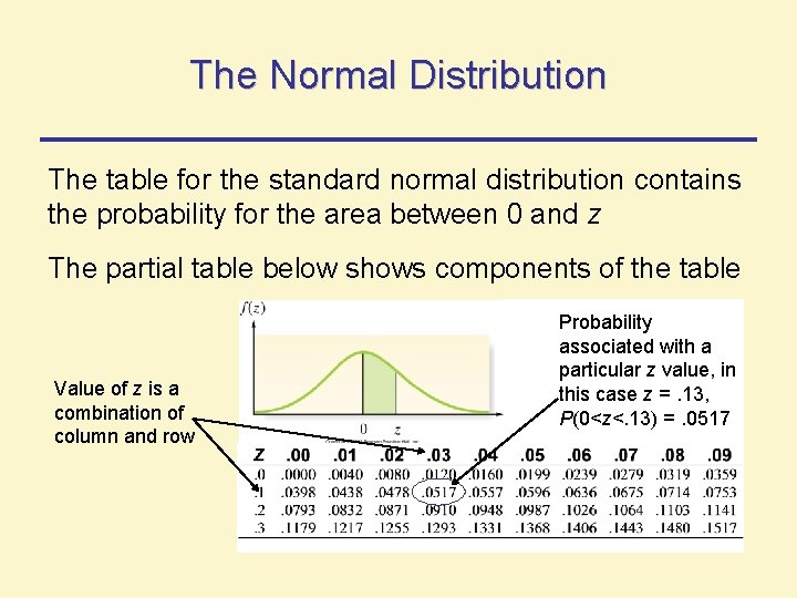
The Normal Distribution The table for the standard normal distribution contains the probability for the area between 0 and z The partial table below shows components of the table Value of z is a combination of column and row Probability associated with a particular z value, in this case z =. 13, P(0<z<. 13) =. 0517

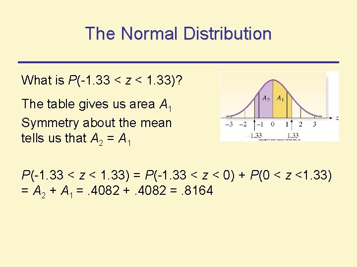
The Normal Distribution What is P(-1. 33 < z < 1. 33)? The table gives us area A 1 Symmetry about the mean tells us that A 2 = A 1 P(-1. 33 < z < 1. 33) = P(-1. 33 < z < 0) + P(0 < z <1. 33) = A 2 + A 1 =. 4082 +. 4082 =. 8164

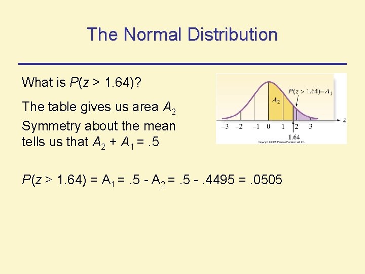
The Normal Distribution What is P(z > 1. 64)? The table gives us area A 2 Symmetry about the mean tells us that A 2 + A 1 =. 5 P(z > 1. 64) = A 1 =. 5 - A 2 =. 5 -. 4495 =. 0505

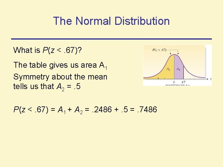
The Normal Distribution What is P(z <. 67)? The table gives us area A 1 Symmetry about the mean tells us that A 2 =. 5 P(z <. 67) = A 1 + A 2 =. 2486 +. 5 =. 7486

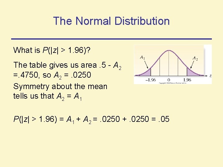
The Normal Distribution What is P(|z| > 1. 96)? The table gives us area. 5 - A 2 =. 4750, so A 2 =. 0250 Symmetry about the mean tells us that A 2 = A 1 P(|z| > 1. 96) = A 1 + A 2 =. 0250 +. 0250 =. 05

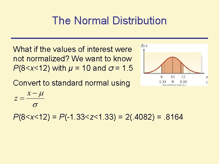
The Normal Distribution What if the values of interest were not normalized? We want to know P(8<x<12) with μ = 10 and σ = 1. 5 Convert to standard normal using P(8<x<12) = P(-1. 33<z<1. 33) = 2(. 4082) =. 8164

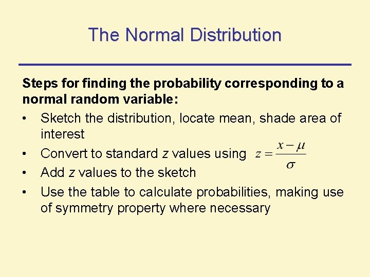
The Normal Distribution Steps for finding the probability corresponding to a normal random variable: • Sketch the distribution, locate mean, shade area of interest • Convert to standard z values using • Add z values to the sketch • Use the table to calculate probabilities, making use of symmetry property where necessary

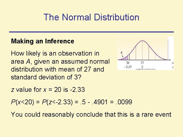
The Normal Distribution Making an Inference How likely is an observation in area A, given an assumed normal distribution with mean of 27 and standard deviation of 3? z value for x = 20 is -2. 33 P(x<20) = P(z<-2. 33) =. 5 -. 4901 =. 0099 You could reasonably conclude that this is a rare event

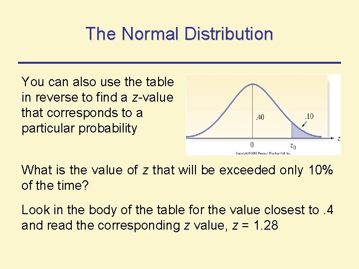
The Normal Distribution You can also use the table in reverse to find a z-value that corresponds to a particular probability What is the value of z that will be exceeded only 10% of the time? Look in the body of the table for the value closest to. 4 and read the corresponding z value, z = 1. 28

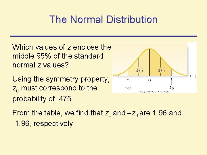
The Normal Distribution Which values of z enclose the middle 95% of the standard normal z values? Using the symmetry property, z 0 must correspond to the probability of. 475 From the table, we find that z 0 and –z 0 are 1. 96 and -1. 96, respectively

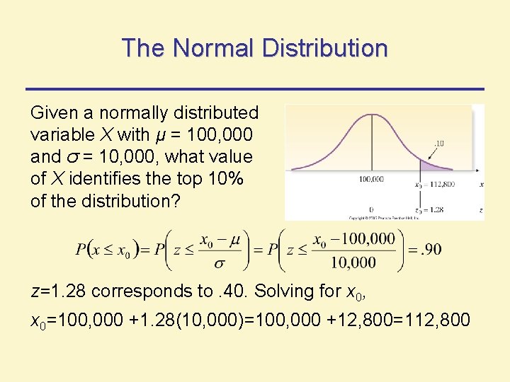
The Normal Distribution Given a normally distributed variable X with μ = 100, 000 and σ = 10, 000, what value of X identifies the top 10% of the distribution? z=1. 28 corresponds to. 40. Solving for x 0, x 0=100, 000 +1. 28(10, 000)=100, 000 +12, 800=112, 800

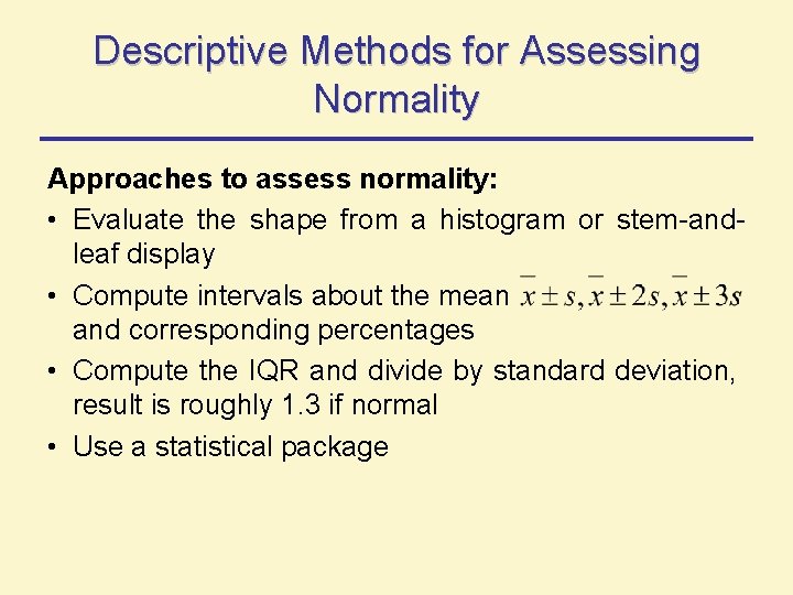
Descriptive Methods for Assessing Normality Approaches to assess normality: • Evaluate the shape from a histogram or stem-andleaf display • Compute intervals about the mean and corresponding percentages • Compute the IQR and divide by standard deviation, result is roughly 1. 3 if normal • Use a statistical package

Approximating a Binomial Distribution with a Normal Distribution You can use a normal distribution as an approximation of a binomial distribution for large values of n Often needed given limitation of binomial tables Need to add a correction for continuity, because of the discrete nature of the binomial distribution Correction is to add. 5 to x when converting to standard z values Interval ( - 3 , + 3 ) should be within the range of the binomial random variable (0 -n) for the normal distribution to be an adequate approximation

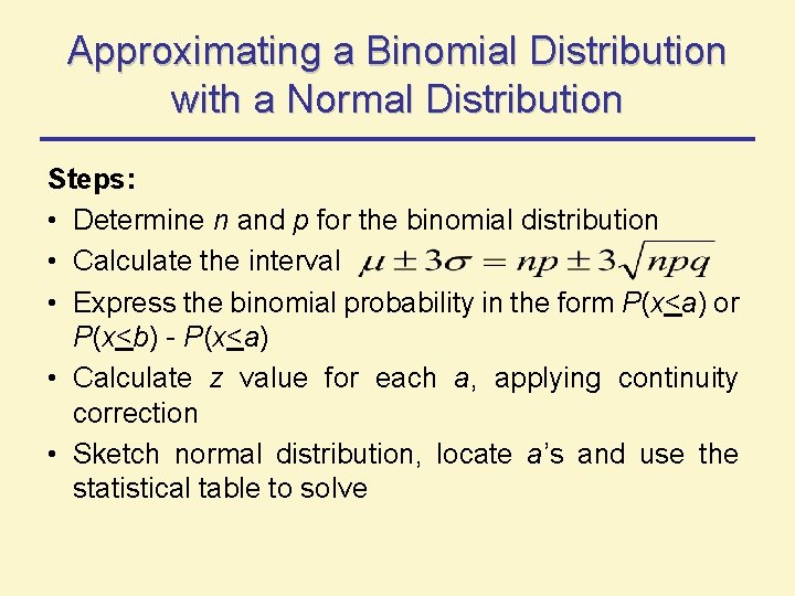
Approximating a Binomial Distribution with a Normal Distribution Steps: • Determine n and p for the binomial distribution • Calculate the interval • Express the binomial probability in the form P(x<a) or P(x<b) - P(x<a) • Calculate z value for each a, applying continuity correction • Sketch normal distribution, locate a’s and use the statistical table to solve