Chapter 4 Continuous Random Variables and Probability Distributions

4. 1 Continuous Random Variables and Probability Distributions

Continuous Random Variables A random variable X is continuous if its set of possible values is an entire interval of numbers (If A < B, then any number x between A and B is possible).

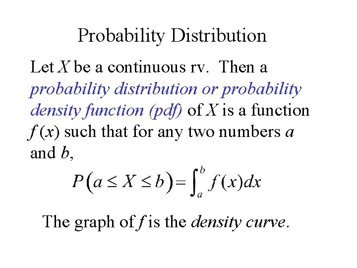
Probability Distribution Let X be a continuous rv. Then a probability distribution or probability density function (pdf) of X is a function f (x) such that for any two numbers a and b, The graph of f is the density curve.

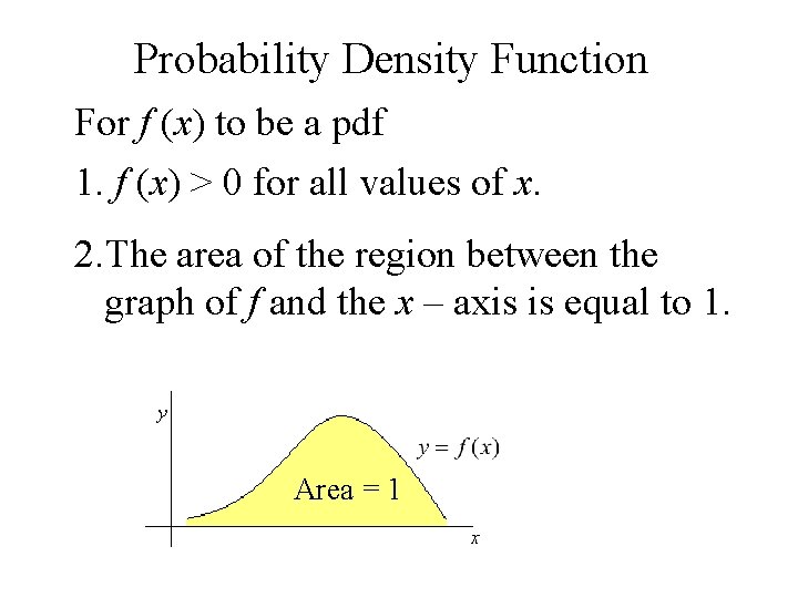
Probability Density Function For f (x) to be a pdf 1. f (x) > 0 for all values of x. 2. The area of the region between the graph of f and the x – axis is equal to 1. Area = 1

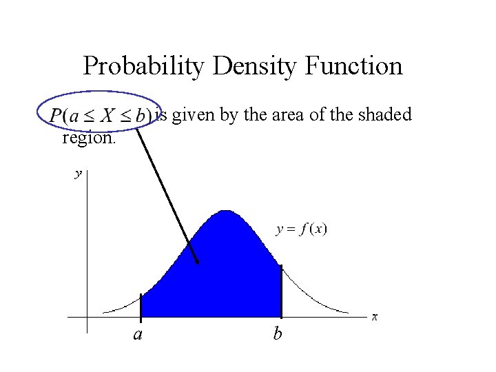
Probability Density Function is given by the area of the shaded region. a b

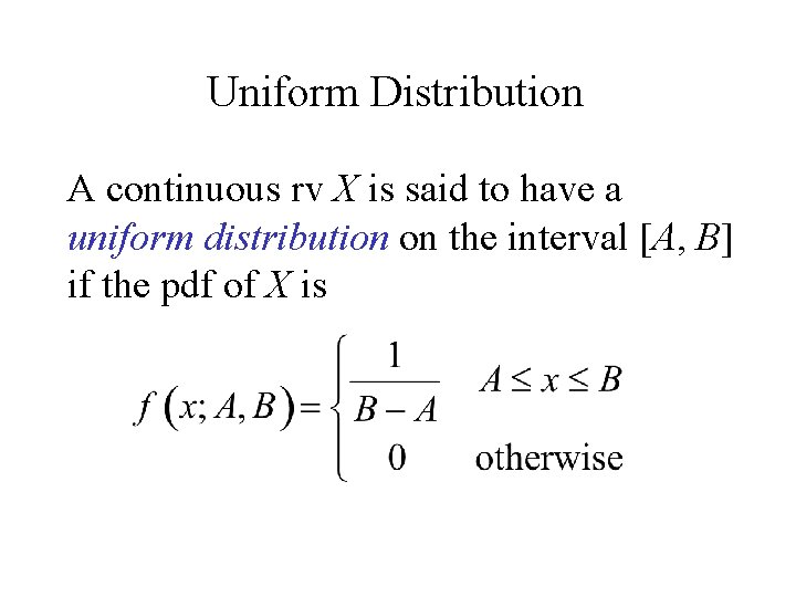
Uniform Distribution A continuous rv X is said to have a uniform distribution on the interval [A, B] if the pdf of X is

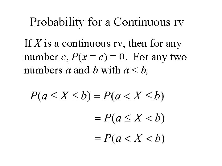
Probability for a Continuous rv If X is a continuous rv, then for any number c, P(x = c) = 0. For any two numbers a and b with a < b,

4. 2 Cumulative Distribution Functions and Expected Values

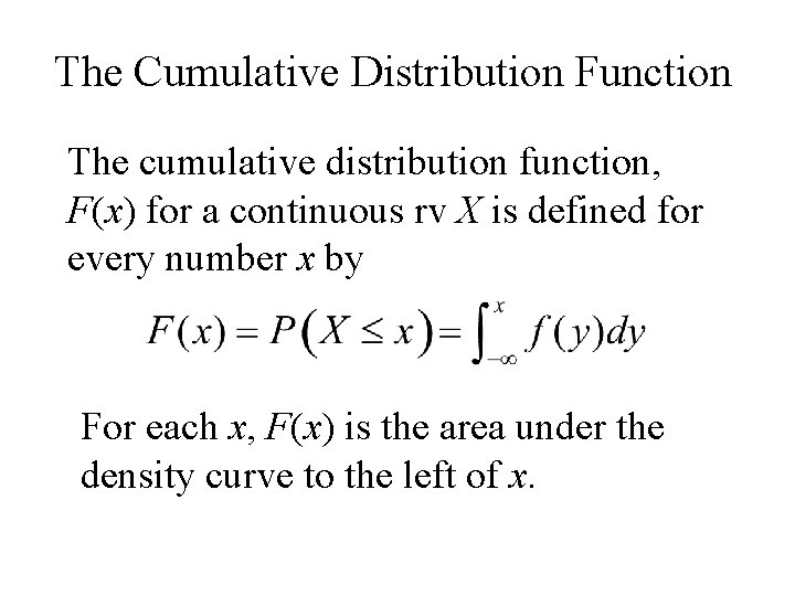
The Cumulative Distribution Function The cumulative distribution function, F(x) for a continuous rv X is defined for every number x by For each x, F(x) is the area under the density curve to the left of x.

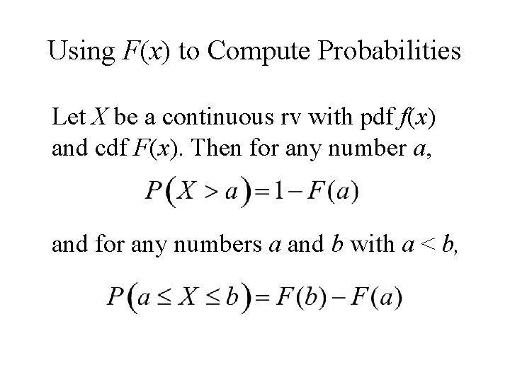
Using F(x) to Compute Probabilities Let X be a continuous rv with pdf f(x) and cdf F(x). Then for any number a, and for any numbers a and b with a < b,

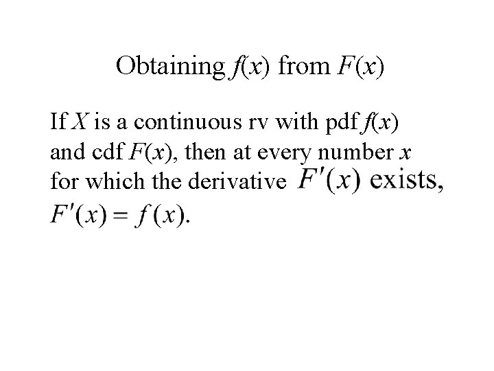
Obtaining f(x) from F(x) If X is a continuous rv with pdf f(x) and cdf F(x), then at every number x for which the derivative

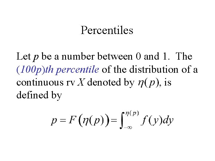
Percentiles Let p be a number between 0 and 1. The (100 p)th percentile of the distribution of a continuous rv X denoted by , is defined by

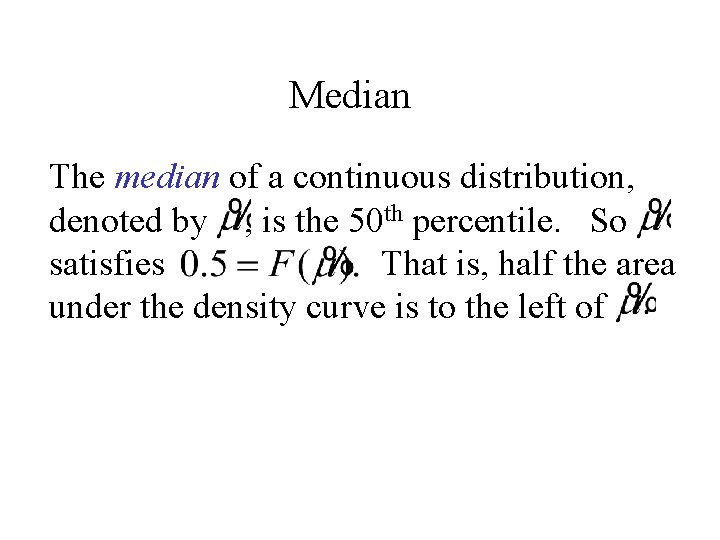
Median The median of a continuous distribution, denoted by , is the 50 th percentile. So satisfies That is, half the area under the density curve is to the left of

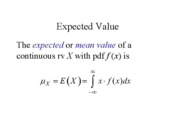
Expected Value The expected or mean value of a continuous rv X with pdf f (x) is

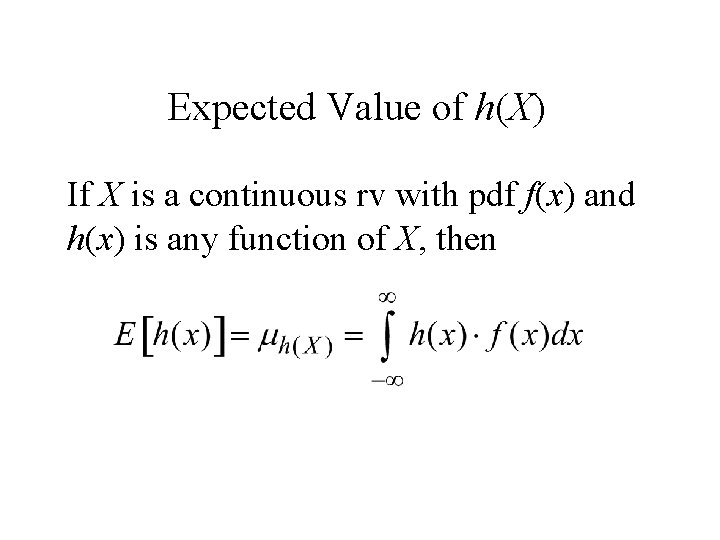
Expected Value of h(X) If X is a continuous rv with pdf f(x) and h(x) is any function of X, then

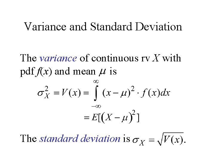
Variance and Standard Deviation The variance of continuous rv X with pdf f(x) and mean is The standard deviation is

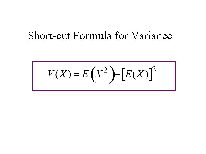
Short-cut Formula for Variance

4. 3 The Normal Distribution

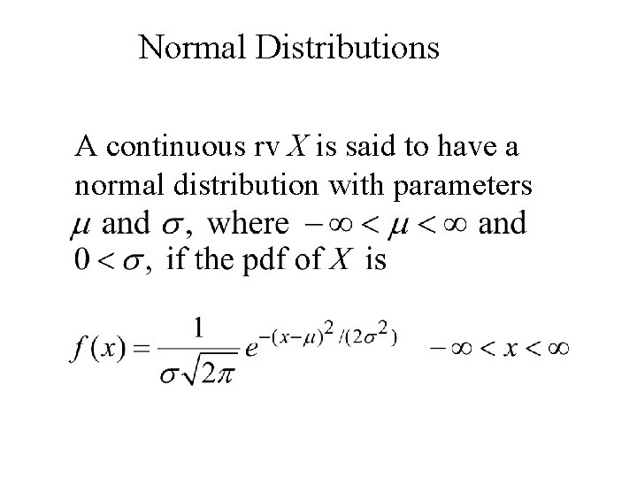
Normal Distributions A continuous rv X is said to have a normal distribution with parameters

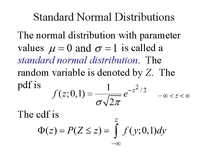
Standard Normal Distributions The normal distribution with parameter values is called a standard normal distribution. The random variable is denoted by Z. The pdf is The cdf is

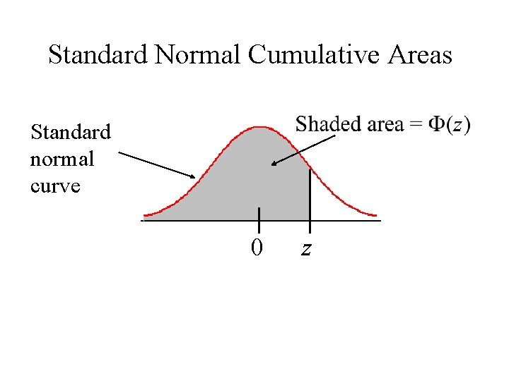
Standard Normal Cumulative Areas Standard normal curve 0 z

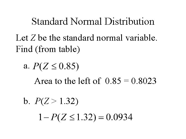
Standard Normal Distribution Let Z be the standard normal variable. Find (from table) a. Area to the left of 0. 85 = 0. 8023 b. P(Z > 1. 32)

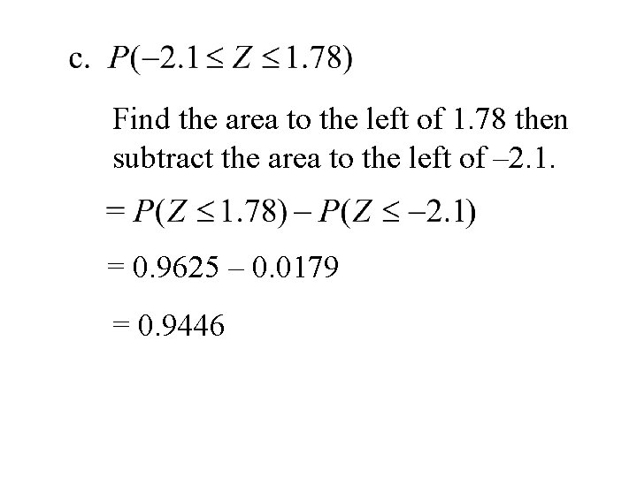
Find the area to the left of 1. 78 then subtract the area to the left of – 2. 1. = 0. 9625 – 0. 0179 = 0. 9446

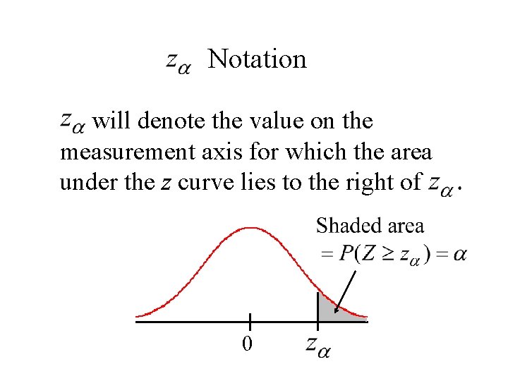
Notation will denote the value on the measurement axis for which the area under the z curve lies to the right of 0

Ex. Let Z be the standard normal variable. Find z if a. P(Z < z) = 0. 9278. Look at the table and find an entry = 0. 9278 then read back to find z = 1. 46. b. P(–z < Z < z) = 0. 8132 P(z < Z < –z ) = 2 P(0 < Z < z) = 2[P(z < Z ) – ½] = 2 P(z < Z ) – 1 = 0. 8132 P(z < Z ) = 0. 9066 z = 1. 32

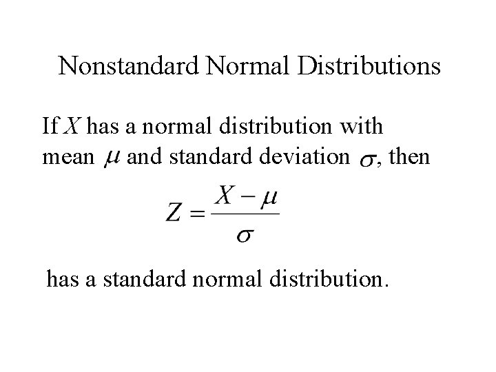
Nonstandard Normal Distributions If X has a normal distribution with mean and standard deviation , then has a standard normal distribution.

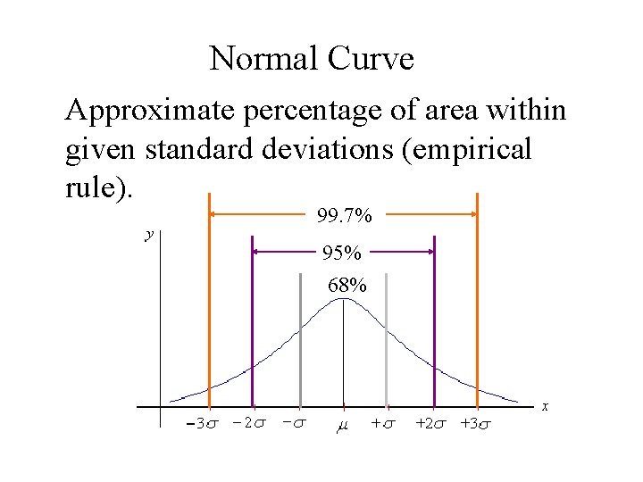
Normal Curve Approximate percentage of area within given standard deviations (empirical rule). 99. 7% 95% 68%

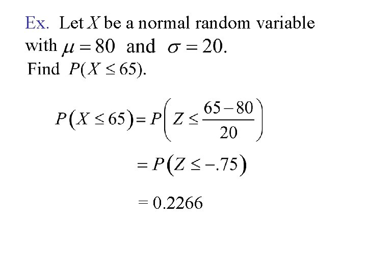
Ex. Let X be a normal random variable with = 0. 2266

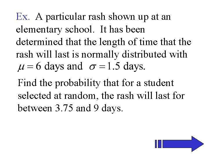
Ex. A particular rash shown up at an elementary school. It has been determined that the length of time that the rash will last is normally distributed with Find the probability that for a student selected at random, the rash will last for between 3. 75 and 9 days.

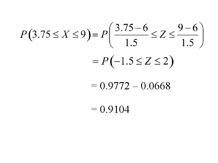
= 0. 9772 – 0. 0668 = 0. 9104

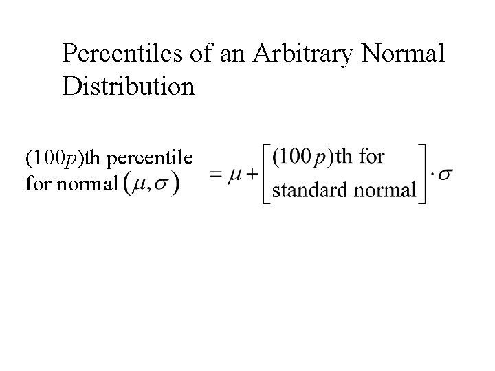
Percentiles of an Arbitrary Normal Distribution (100 p)th percentile for normal

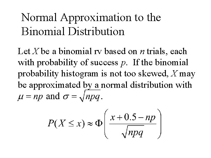
Normal Approximation to the Binomial Distribution Let X be a binomial rv based on n trials, each with probability of success p. If the binomial probability histogram is not too skewed, X may be approximated by a normal distribution with

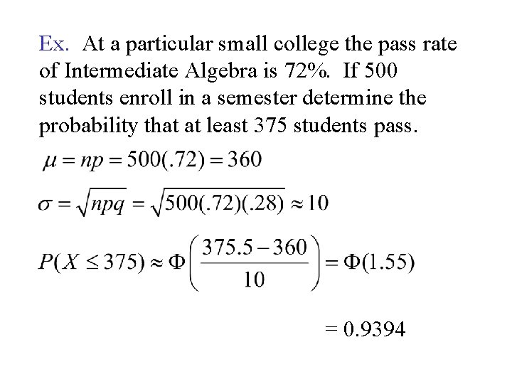
Ex. At a particular small college the pass rate of Intermediate Algebra is 72%. If 500 students enroll in a semester determine the probability that at least 375 students pass. = 0. 9394

4. 4 The Gamma Distribution and Its Relatives

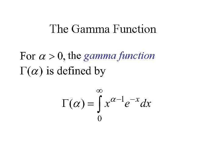
The Gamma Function the gamma function

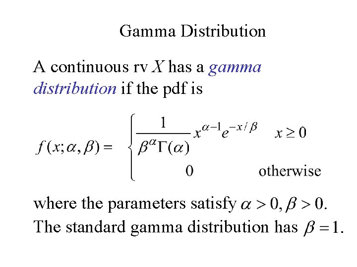
Gamma Distribution A continuous rv X has a gamma distribution if the pdf is where the parameters satisfy The standard gamma distribution has

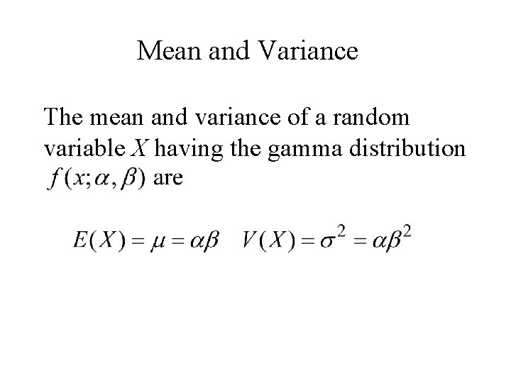
Mean and Variance The mean and variance of a random variable X having the gamma distribution

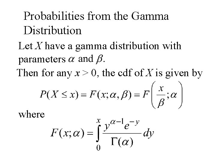
Probabilities from the Gamma Distribution Let X have a gamma distribution with parameters Then for any x > 0, the cdf of X is given by where

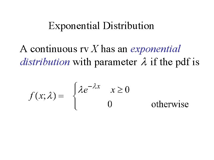
Exponential Distribution A continuous rv X has an exponential distribution with parameter if the pdf is

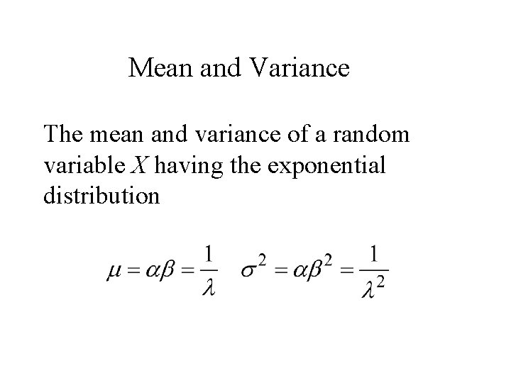
Mean and Variance The mean and variance of a random variable X having the exponential distribution

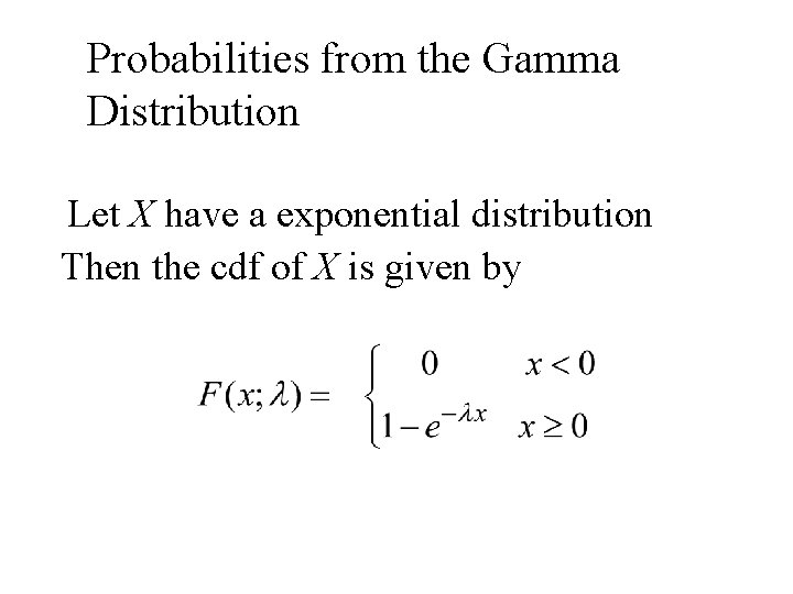
Probabilities from the Gamma Distribution Let X have a exponential distribution Then the cdf of X is given by

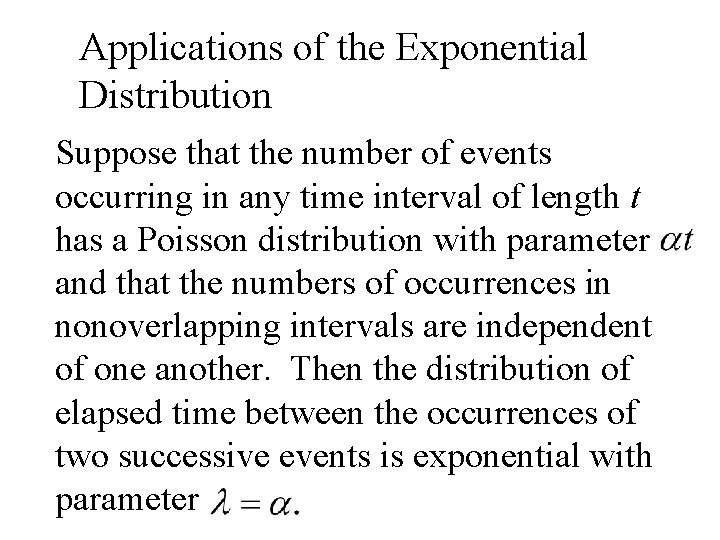
Applications of the Exponential Distribution Suppose that the number of events occurring in any time interval of length t has a Poisson distribution with parameter and that the numbers of occurrences in nonoverlapping intervals are independent of one another. Then the distribution of elapsed time between the occurrences of two successive events is exponential with parameter

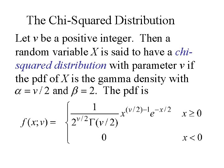
The Chi-Squared Distribution Let v be a positive integer. Then a random variable X is said to have a chisquared distribution with parameter v if the pdf of X is the gamma density with The pdf is

The Chi-Squared Distribution The parameter v is called the number of degrees of freedom (df) of X. The symbol is often used in place of “chisquared. ”

4. 5 Other Continuous Distributions

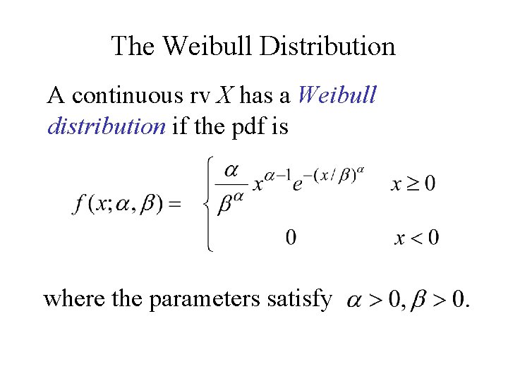
The Weibull Distribution A continuous rv X has a Weibull distribution if the pdf is where the parameters satisfy

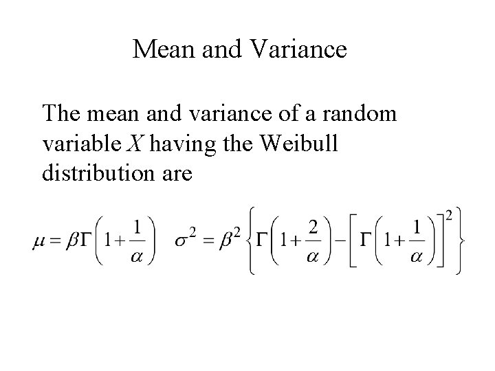
Mean and Variance The mean and variance of a random variable X having the Weibull distribution are

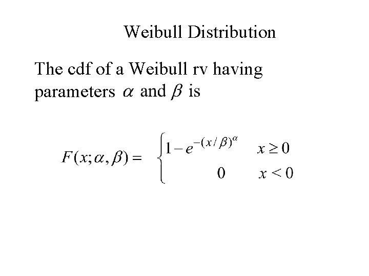
Weibull Distribution The cdf of a Weibull rv having parameters

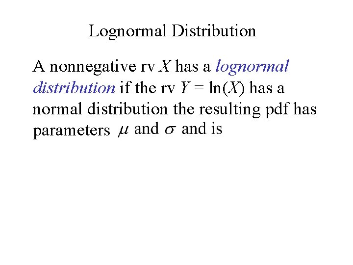
Lognormal Distribution A nonnegative rv X has a lognormal distribution if the rv Y = ln(X) has a normal distribution the resulting pdf has parameters

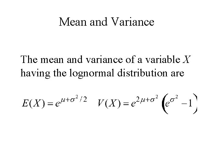
Mean and Variance The mean and variance of a variable X having the lognormal distribution are

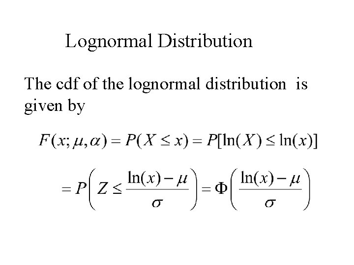
Lognormal Distribution The cdf of the lognormal distribution is given by

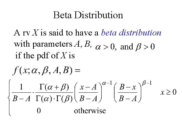
Beta Distribution A rv X is said to have a beta distribution with parameters A, B, if the pdf of X is

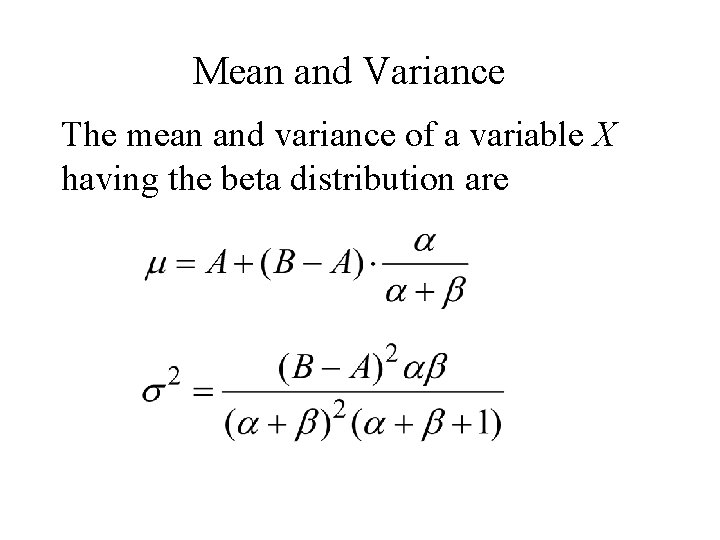
Mean and Variance The mean and variance of a variable X having the beta distribution are

4. 6 Probability Plots

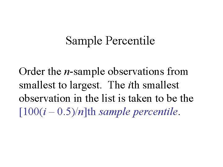
Sample Percentile Order the n-sample observations from smallest to largest. The ith smallest observation in the list is taken to be the [100(i – 0. 5)/n]th sample percentile.

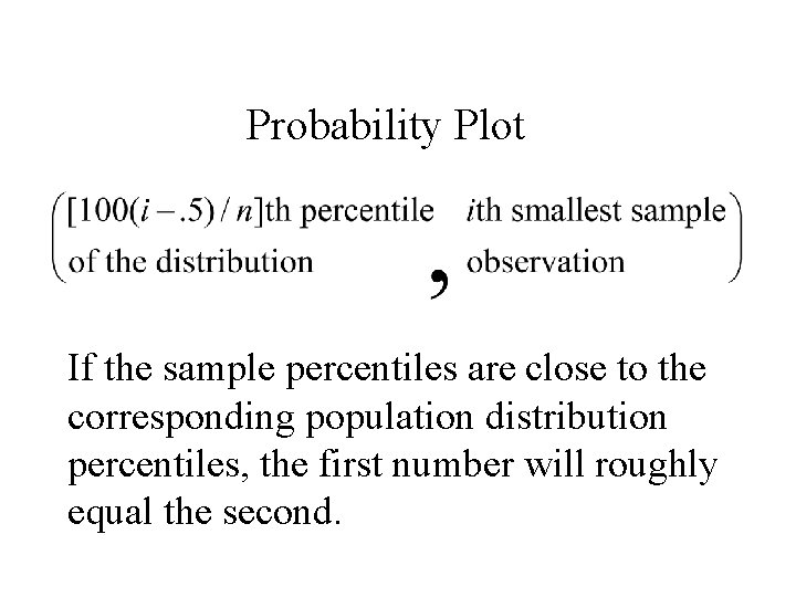
Probability Plot If the sample percentiles are close to the corresponding population distribution percentiles, the first number will roughly equal the second.

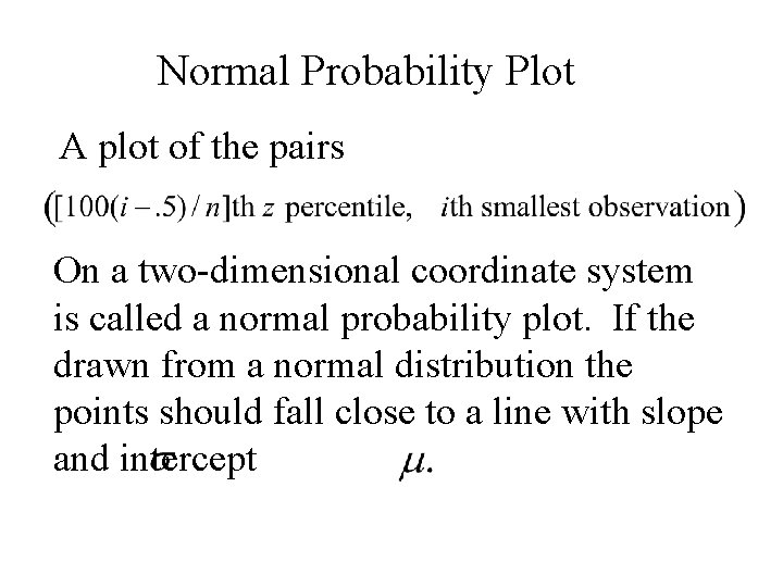
Normal Probability Plot A plot of the pairs On a two-dimensional coordinate system is called a normal probability plot. If the drawn from a normal distribution the points should fall close to a line with slope and intercept

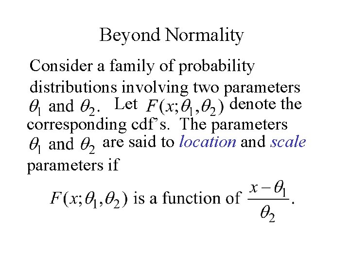
Beyond Normality Consider a family of probability distributions involving two parameters Let denote the corresponding cdf’s. The parameters are said to location and scale parameters if