Chapter 4 Basic Estimation Techniques 2016 by Mc

Chapter 4 Basic Estimation Techniques © 2016 by Mc. Graw-Hill Education. This is proprietary material solely for authorized instructor use. Not authorized for sale or distribution in any manner. This document may not be copied, scanned, duplicated, forwarded, distributed, or posted on a website, in whole or part. 1 -1

Learning Objectives v Set up and interpret simple linear regression equations v Estimate intercept and slope parameters of a regression line using the method of least‐squares v Determine statistical significance using either t‐tests or p‐values associated with parameter estimates v Evaluate the “fit” of a regression equation to the data using the R 2 statistic and test for statistical significance of the whole regression equation using an F‐test v Set up and interpret multiple regression models v Use linear regression techniques to estimate the parameters of two common nonlinear models: quadratic and log‐linear regression models © 2016 by Mc. Graw-Hill Education. This is proprietary material solely for authorized instructor use. Not authorized for sale or distribution in any manner. This document may not be copied, scanned, duplicated, forwarded, distributed, or posted on a website, in whole or part. 4 -2

Basic Estimation v Parameters ~ The coefficients in an equation that determine the exact mathematical relation among the variables v Parameter estimation ~ The process of finding estimates of the numerical values of the parameters of an equation © 2016 by Mc. Graw-Hill Education. This is proprietary material solely for authorized instructor use. Not authorized for sale or distribution in any manner. This document may not be copied, scanned, duplicated, forwarded, distributed, or posted on a website, in whole or part. 4 -3

Regression Analysis v Regression analysis ~ A statistical technique for estimating the parameters of an equation and testing for statistical significance v Dependent variable ~ Variable whose variation is to be explained v Explanatory variables ~ Variables that are thought to cause the dependent variable to take on different values © 2016 by Mc. Graw-Hill Education. This is proprietary material solely for authorized instructor use. Not authorized for sale or distribution in any manner. This document may not be copied, scanned, duplicated, forwarded, distributed, or posted on a website, in whole or part. 4 -4

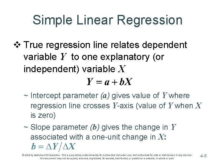
Simple Linear Regression v True regression line relates dependent variable Y to one explanatory (or independent) variable X ~ Intercept parameter (a) gives value of Y where regression line crosses Y-axis (value of Y when X is zero) ~ Slope parameter (b) gives the change in Y associated with a one-unit change in X: © 2016 by Mc. Graw-Hill Education. This is proprietary material solely for authorized instructor use. Not authorized for sale or distribution in any manner. This document may not be copied, scanned, duplicated, forwarded, distributed, or posted on a website, in whole or part. 4 -5

Simple Linear Regression v Regression line shows the average or expected value of Y for each level of X v True (or actual) underlying relation between Y and X is unknown to the researcher but is to be discovered by analyzing the sample data v Random error term ~ Unobservable term added to a regression model to capture the effects of all the minor, unpredictable factors that affect Y but cannot reasonably by included as explanatory variables © 2016 by Mc. Graw-Hill Education. This is proprietary material solely for authorized instructor use. Not authorized for sale or distribution in any manner. This document may not be copied, scanned, duplicated, forwarded, distributed, or posted on a website, in whole or part. 4 -6

Fitting a Regression Line v Time series ~ A data set in which the data for the dependent and explanatory variables are collected over time for a single firm v Cross-sectional ~ A data set in which the data for the dependent and explanatory variables are collected from many different firms or industries at a given point in time © 2016 by Mc. Graw-Hill Education. This is proprietary material solely for authorized instructor use. Not authorized for sale or distribution in any manner. This document may not be copied, scanned, duplicated, forwarded, distributed, or posted on a website, in whole or part. 4 -7

Fitting a Regression Line v Method of least squares ~ A method of estimating the parameters of a linear regression equation by finding the line that minimizes the sum of the squared distances from each sample data point to the sample regression line © 2016 by Mc. Graw-Hill Education. This is proprietary material solely for authorized instructor use. Not authorized for sale or distribution in any manner. This document may not be copied, scanned, duplicated, forwarded, distributed, or posted on a website, in whole or part. 4 -8

Fitting a Regression Line v Parameter estimates are obtained by choosing values of a & b that minimize the sum of squared residuals ~ The residual is the difference between the actual and fitted values of Y: Yi – Ŷi ~ Equivalent to fitting a line through a scatter diagram of the sample data points © 2016 by Mc. Graw-Hill Education. This is proprietary material solely for authorized instructor use. Not authorized for sale or distribution in any manner. This document may not be copied, scanned, duplicated, forwarded, distributed, or posted on a website, in whole or part. 4 -9

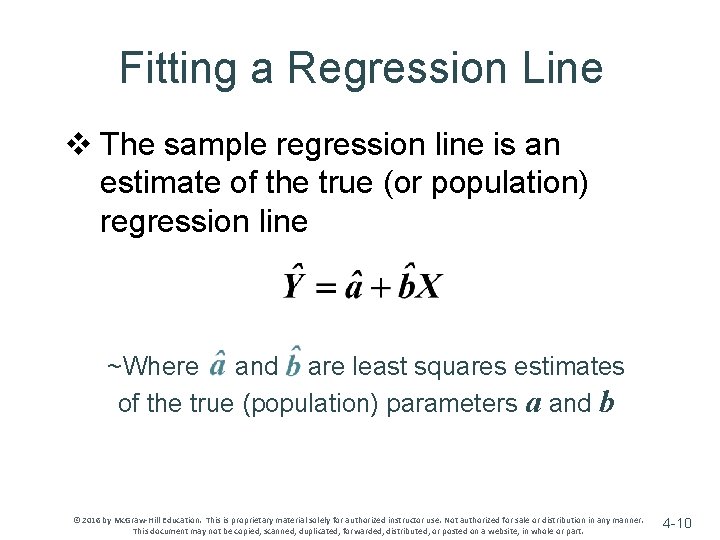
Fitting a Regression Line v The sample regression line is an estimate of the true (or population) regression line ~Where and are least squares estimates of the true (population) parameters a and b © 2016 by Mc. Graw-Hill Education. This is proprietary material solely for authorized instructor use. Not authorized for sale or distribution in any manner. This document may not be copied, scanned, duplicated, forwarded, distributed, or posted on a website, in whole or part. 4 -10

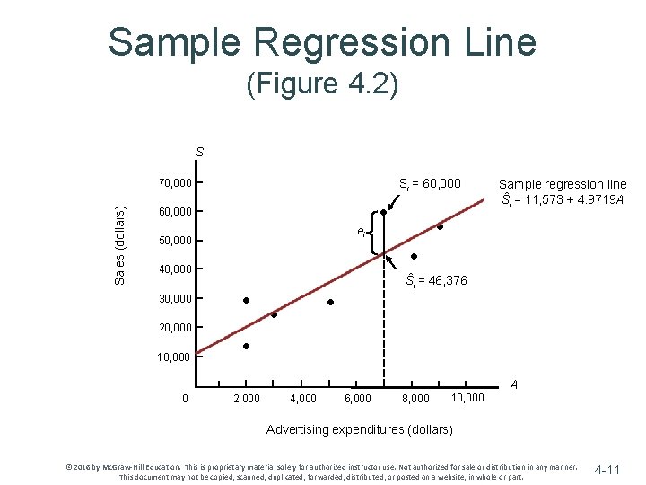
Sample Regression Line (Figure 4. 2) S Si = 60, 000 Sales (dollars) 70, 000 60, 000 ei 50, 000 20, 000 10, 000 • • 40, 000 30, 000 • Sample regression line Ŝi = 11, 573 + 4. 9719 A • Ŝi = 46, 376 • • • A 0 2, 000 4, 000 6, 000 8, 000 10, 000 Advertising expenditures (dollars) © 2016 by Mc. Graw-Hill Education. This is proprietary material solely for authorized instructor use. Not authorized for sale or distribution in any manner. This document may not be copied, scanned, duplicated, forwarded, distributed, or posted on a website, in whole or part. 4 -11

Unbiased Estimators v The estimates & do not generally equal the true values of a & b ~ & are random variables computed using data from a random sample v The distribution of values the estimates might take is centered around the true value of the parameter v An estimator is unbiased if its average value (or expected value) is equal to the true value of the parameter © 2016 by Mc. Graw-Hill Education. This is proprietary material solely for authorized instructor use. Not authorized for sale or distribution in any manner. This document may not be copied, scanned, duplicated, forwarded, distributed, or posted on a website, in whole or part. 4 -12

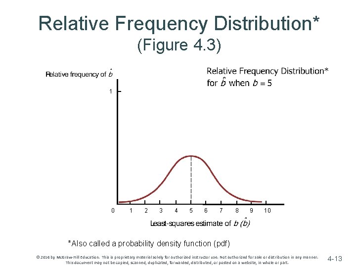
Relative Frequency Distribution* (Figure 4. 3) 1 0 1 2 3 4 5 6 7 8 9 10 *Also called a probability density function (pdf) © 2016 by Mc. Graw-Hill Education. This is proprietary material solely for authorized instructor use. Not authorized for sale or distribution in any manner. This document may not be copied, scanned, duplicated, forwarded, distributed, or posted on a website, in whole or part. 4 -13

Statistical Significance v Statistical significance ~ There is sufficient evidence from the sample to indicate that the true value of the coefficient is not zero v Hypothesis testing ~ A statistical technique for making a probabilistic statement about the true value of a parameter © 2016 by Mc. Graw-Hill Education. This is proprietary material solely for authorized instructor use. Not authorized for sale or distribution in any manner. This document may not be copied, scanned, duplicated, forwarded, distributed, or posted on a website, in whole or part. 4 -14

Statistical Significance v Must determine if there is sufficient statistical evidence to indicate that Y is truly related to X (i. e. , b 0) v Even if b = 0, it is possible that the sample will produce an estimate that is different from zero v Test for statistical significance using -tests or p-values © 2016 by Mc. Graw-Hill Education. This is proprietary material solely for authorized instructor use. Not authorized for sale or distribution in any manner. This document may not be copied, scanned, duplicated, forwarded, distributed, or posted on a website, in whole or part. t 4 -15

Statistical Significance v First determine the level of significance ~ Probability of finding a parameter estimate to be statistically different from zero when, in fact, it is zero ~ Probability of a Type I Error v 1 – level of significance = level of confidence ~ Level of confidence is the probability of correctly failing to reject the true hypothesis that b = 0 © 2016 by Mc. Graw-Hill Education. This is proprietary material solely for authorized instructor use. Not authorized for sale or distribution in any manner. This document may not be copied, scanned, duplicated, forwarded, distributed, or posted on a website, in whole or part. 4 -16

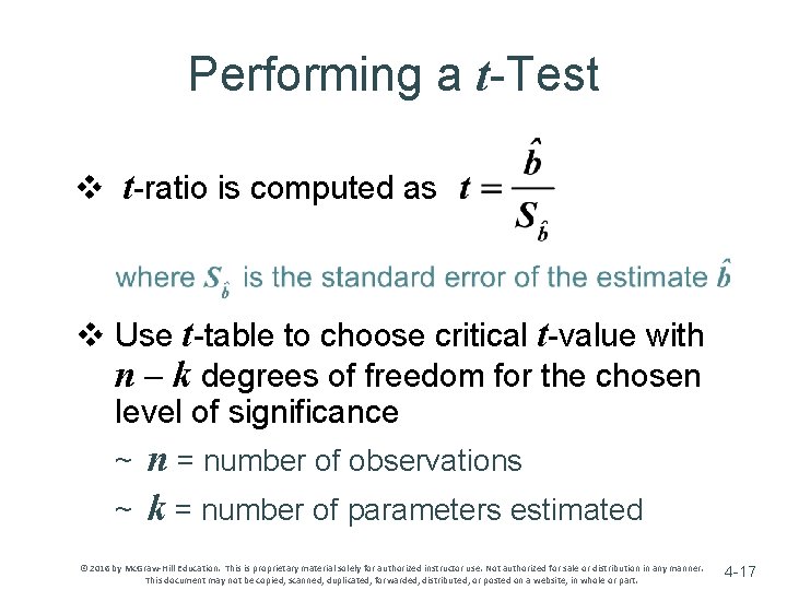
Performing a t-Test v t-ratio is computed as v Use t-table to choose critical t-value with n – k degrees of freedom for the chosen level of significance ~ n = number of observations ~ k = number of parameters estimated © 2016 by Mc. Graw-Hill Education. This is proprietary material solely for authorized instructor use. Not authorized for sale or distribution in any manner. This document may not be copied, scanned, duplicated, forwarded, distributed, or posted on a website, in whole or part. 4 -17

Performing a t-Test v t-statistic ~ Numerical value of the t-ratio v If the absolute value of t-statistic is greater than the critical t, the parameter estimate is statistically significant at the given level of significance © 2016 by Mc. Graw-Hill Education. This is proprietary material solely for authorized instructor use. Not authorized for sale or distribution in any manner. This document may not be copied, scanned, duplicated, forwarded, distributed, or posted on a website, in whole or part. 4 -18

Using p-Values v Treat as statistically significant only those parameter estimates with p-values smaller than the maximum acceptable significance level v p-value gives exact level of significance ~ Also the probability of finding significance when none exists © 2016 by Mc. Graw-Hill Education. This is proprietary material solely for authorized instructor use. Not authorized for sale or distribution in any manner. This document may not be copied, scanned, duplicated, forwarded, distributed, or posted on a website, in whole or part. 4 -19

Coefficient of Determination v R 2 measures the fraction of total variation in the dependent variable (Y) that is explained by the variation in X ~ Ranges from 0 to 1 ~ High R 2 indicates Y and X are highly correlated, and does not prove that Y and X are causally related © 2016 by Mc. Graw-Hill Education. This is proprietary material solely for authorized instructor use. Not authorized for sale or distribution in any manner. This document may not be copied, scanned, duplicated, forwarded, distributed, or posted on a website, in whole or part. 4 -20

F-Test v Used to test for significance of overall regression equation v Compare F-statistic to critical F-value from F-table ~ Two degrees of freedom, n – k & k – 1 ~ Level of significance v If F-statistic exceeds the critical F, the regression equation overall is statistically significant at the specified level of significance © 2016 by Mc. Graw-Hill Education. This is proprietary material solely for authorized instructor use. Not authorized for sale or distribution in any manner. This document may not be copied, scanned, duplicated, forwarded, distributed, or posted on a website, in whole or part. 4 -21

Multiple Regression v Uses more than one explanatory variable v Coefficient for each explanatory variable measures the change in the dependent variable associated with a one-unit change in that explanatory variable, all else constant © 2016 by Mc. Graw-Hill Education. This is proprietary material solely for authorized instructor use. Not authorized for sale or distribution in any manner. This document may not be copied, scanned, duplicated, forwarded, distributed, or posted on a website, in whole or part. 4 -22

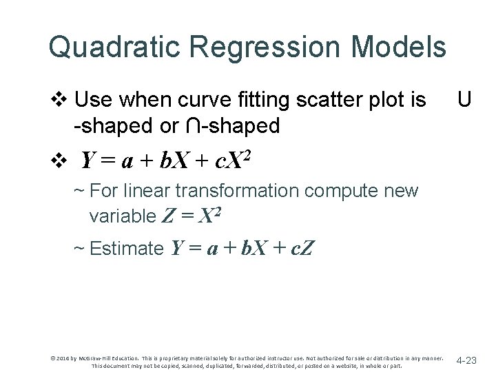
Quadratic Regression Models v Use when curve fitting scatter plot is -shaped or ∩-shaped U v Y = a + b. X + c. X 2 ~ For linear transformation compute new variable Z = X 2 ~ Estimate Y = a + b. X + c. Z © 2016 by Mc. Graw-Hill Education. This is proprietary material solely for authorized instructor use. Not authorized for sale or distribution in any manner. This document may not be copied, scanned, duplicated, forwarded, distributed, or posted on a website, in whole or part. 4 -23

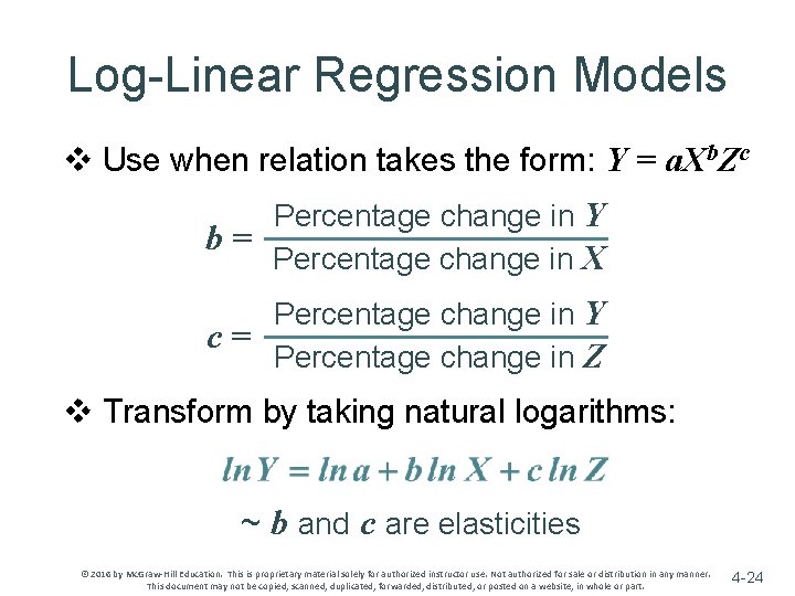
Log-Linear Regression Models v Use when relation takes the form: Y = a. Xb. Zc Percentage change in Y b= Percentage change in X Percentage change in Y c= Percentage change in Z v Transform by taking natural logarithms: ~ b and c are elasticities © 2016 by Mc. Graw-Hill Education. This is proprietary material solely for authorized instructor use. Not authorized for sale or distribution in any manner. This document may not be copied, scanned, duplicated, forwarded, distributed, or posted on a website, in whole or part. 4 -24

Summary v A simple linear regression model relates a dependent variable Y to a single explanatory variable X ~ The regression equation is correctly interpreted as providing the average value (expected value) of Y for a given value of X v Parameter estimates are obtained by choosing values of a and b that create the best-fitting line that passes through the scatter diagram of the sample data points v If the absolute value of the t-ratio is greater (less) than the critical t-value, then is (is not) statistically significant ~ Exact level of significance associated with a t-statistic is its p-value v A high R 2 indicates Y and X are highly correlated and the data tightly fit the sample regression line © 2016 by Mc. Graw-Hill Education. This is proprietary material solely for authorized instructor use. Not authorized for sale or distribution in any manner. This document may not be copied, scanned, duplicated, forwarded, distributed, or posted on a website, in whole or part. 4 -25

Summary v If the F-statistic exceeds the critical F-value, the regression equation is statistically significant v In multiple regression, the coefficients measure the change in Y associated with a one-unit change in that explanatory variable v Quadratic regression models are appropriate when the curve fitting the scatter plot is U-shaped or ∩-shaped (Y = a + b. X + c. X 2) v Log-linear regression models are appropriate when the relation is in multiplicative exponential form (Y = a. Xb. Zc) ~ The equation is transformed by taking natural logarithms © 2016 by Mc. Graw-Hill Education. This is proprietary material solely for authorized instructor use. Not authorized for sale or distribution in any manner. This document may not be copied, scanned, duplicated, forwarded, distributed, or posted on a website, in whole or part. 4 -26