Chapter 4 Algorithm Analysis complexity Investigates computational complexity

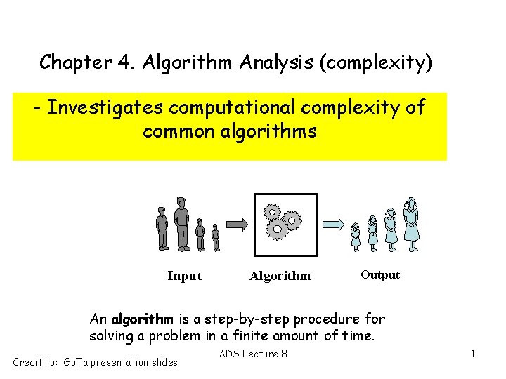
Chapter 4. Algorithm Analysis (complexity) - Investigates computational complexity of common algorithms Input Algorithm Output An algorithm is a step-by-step procedure for solving a problem in a finite amount of time. Credit to: Go. Ta presentation slides. ADS Lecture 8 1

What affects runtime of a program? • the machine it runs on • the programming language • the efficiency of the compiler • the size of the input • the efficiency/complexity of the algorithm? What has the greatest effect?

What affects runtime of an algorithm? • the size of the input • the efficiency/complexity of the algorithm? We measure the number of times the “principal activity” of the algorithm is executed for a given input size n One easy to understand example is search, finding a piece of data in a data set N is the size of the data set “principal activity” might be comparison of key with data What are we interested in? Best case, average case, or worst case?

What affects runtime of an algorithm? Therefore we express the complexity of an algorithm as a function of the size of the input This function tells how the number of times the “principal activity” performed grows as the input size grows. This does not give us an exact figure, but a growth rate. This allows us to compare algorithms theoretically

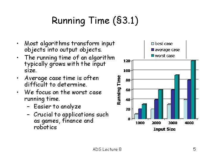
Running Time (§ 3. 1) • Most algorithms transform input objects into output objects. • The running time of an algorithm typically grows with the input size. • Average case time is often difficult to determine. • We focus on the worst case running time. – Easier to analyze – Crucial to applications such as games, finance and robotics ADS Lecture 8 5

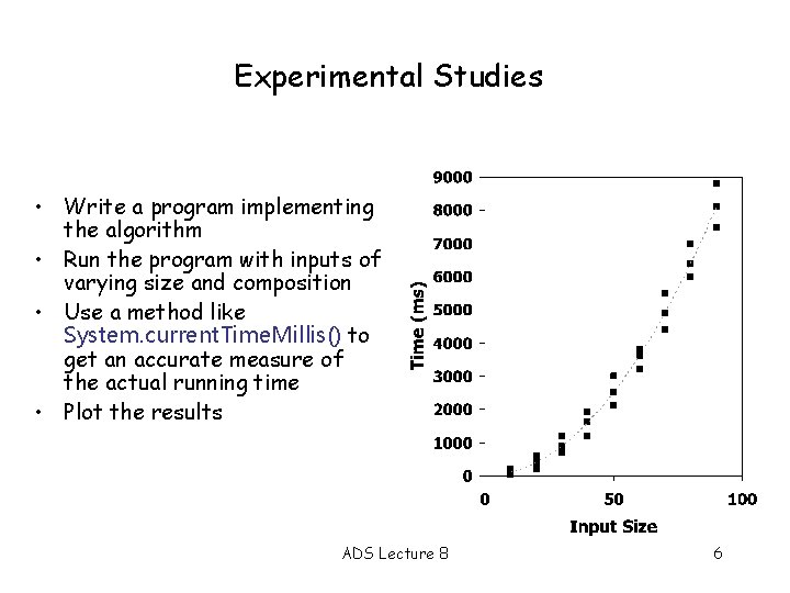
Experimental Studies • Write a program implementing the algorithm • Run the program with inputs of varying size and composition • Use a method like System. current. Time. Millis() to get an accurate measure of the actual running time • Plot the results ADS Lecture 8 6

Limitations of Experiments • It is necessary to implement the algorithm, which may be difficult • Results may not be indicative of the running time on other inputs not included in the experiment. • In order to compare two algorithms, the same hardware and software environments must be used Theoretical Analysis • Uses a high-level description of the algorithm instead of an implementation • Characterizes running time as a function of the input size, n. • Takes into account all possible inputs • Allows us to evaluate the speed of an algorithm independent of the hardware/software environment ADS Lecture 8 7

Primitive Operations • Basic computations performed by an algorithm • Identifiable in pseudocode • Largely independent from the programming language • Exact definition not important (we will see why later) • Assumed to take a constant amount of time ADS Lecture 8 • Examples: – Evaluating an expression – Assigning a value to a variable – Indexing into an array – Calling a method – Returning from a method 8

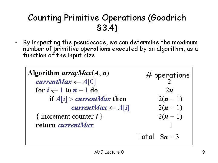
Counting Primitive Operations (Goodrich § 3. 4) • By inspecting the pseudocode, we can determine the maximum number of primitive operations executed by an algorithm, as a function of the input size Algorithm array. Max(A, n) current. Max A[0] for i 1 to n 1 do if A[i] current. Max then current. Max A[i] { increment counter i } return current. Max # operations 2 2 n 2(n 1) 1 Total 8 n 3 ADS Lecture 8 9

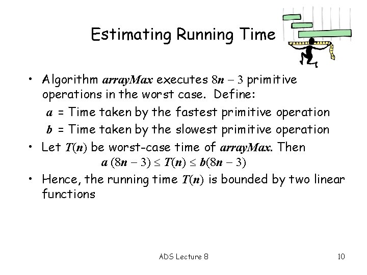
Estimating Running Time • Algorithm array. Max executes 8 n 3 primitive operations in the worst case. Define: a = Time taken by the fastest primitive operation b = Time taken by the slowest primitive operation • Let T(n) be worst-case time of array. Max. Then a (8 n 3) T(n) b(8 n 3) • Hence, the running time T(n) is bounded by two linear functions ADS Lecture 8 10

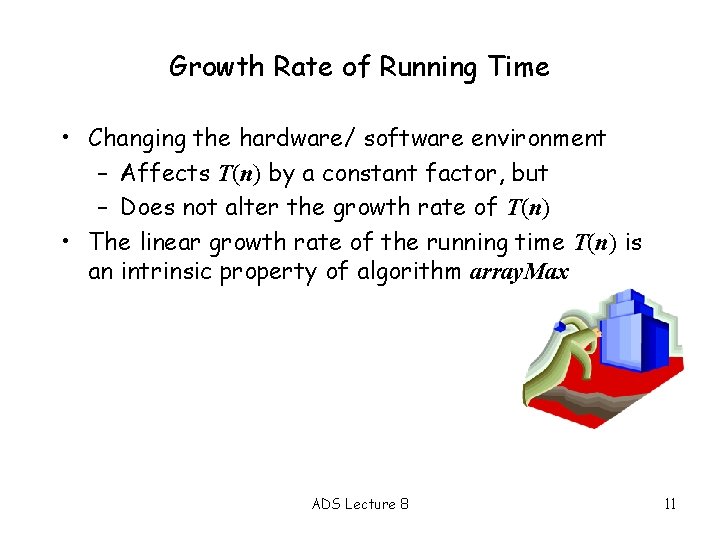
Growth Rate of Running Time • Changing the hardware/ software environment – Affects T(n) by a constant factor, but – Does not alter the growth rate of T(n) • The linear growth rate of the running time T(n) is an intrinsic property of algorithm array. Max ADS Lecture 8 11

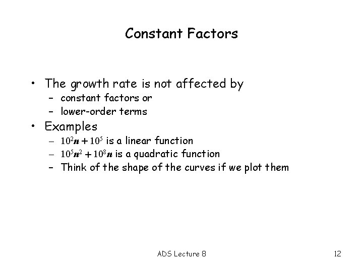
Constant Factors • The growth rate is not affected by – constant factors or – lower-order terms • Examples – 102 n + 105 is a linear function – 105 n 2 + 108 n is a quadratic function – Think of the shape of the curves if we plot them ADS Lecture 8 12

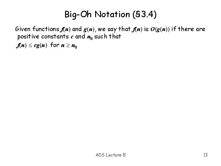
Big-Oh Notation (§ 3. 4) Given functions f(n) and g(n), we say that f(n) is O(g(n)) if there are positive constants c and n 0 such that f(n) cg(n) for n n 0 ADS Lecture 8 13

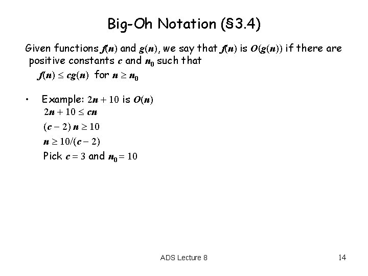
Big-Oh Notation (§ 3. 4) Given functions f(n) and g(n), we say that f(n) is O(g(n)) if there are positive constants c and n 0 such that f(n) cg(n) for n n 0 • Example: 2 n + 10 is O(n) 2 n + 10 cn (c 2) n 10/(c 2) Pick c = 3 and n 0 = 10 ADS Lecture 8 14

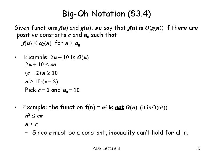
Big-Oh Notation (§ 3. 4) Given functions f(n) and g(n), we say that f(n) is O(g(n)) if there are positive constants c and n 0 such that f(n) cg(n) for n n 0 • Example: 2 n + 10 is O(n) 2 n + 10 cn (c 2) n 10/(c 2) Pick c = 3 and n 0 = 10 • Example: the function f(n) = n 2 is not O(n) (it is O(n 2)) n 2 cn n c – Since c must be a constant, inequality can’t hold for all n. ADS Lecture 8 15

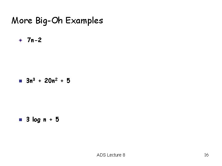
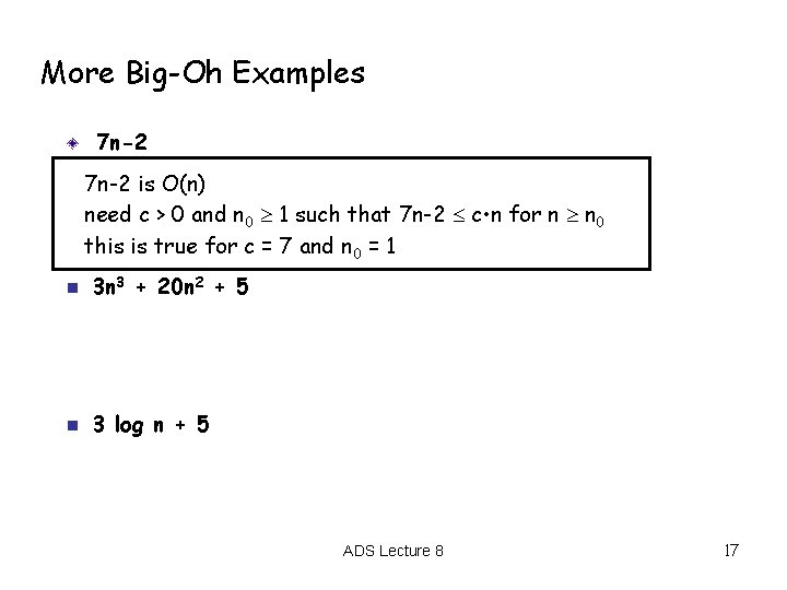
More Big-Oh Examples 7 n-2 n 3 n 3 + 20 n 2 + 5 n 3 log n + 5 ADS Lecture 8 16

More Big-Oh Examples 7 n-2 is O(n) need c > 0 and n 0 1 such that 7 n-2 c • n for n n 0 this is true for c = 7 and n 0 = 1 n 3 n 3 + 20 n 2 + 5 n 3 log n + 5 ADS Lecture 8 17

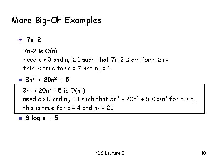
More Big-Oh Examples 7 n-2 is O(n) need c > 0 and n 0 1 such that 7 n-2 c • n for n n 0 this is true for c = 7 and n 0 = 1 n 3 n 3 + 20 n 2 + 5 is O(n 3) need c > 0 and n 0 1 such that 3 n 3 + 20 n 2 + 5 c • n 3 for n n 0 this is true for c = 4 and n 0 = 21 n 3 log n + 5 ADS Lecture 8 18

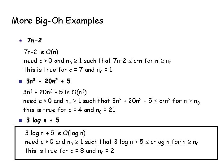
More Big-Oh Examples 7 n-2 is O(n) need c > 0 and n 0 1 such that 7 n-2 c • n for n n 0 this is true for c = 7 and n 0 = 1 n 3 n 3 + 20 n 2 + 5 is O(n 3) need c > 0 and n 0 1 such that 3 n 3 + 20 n 2 + 5 c • n 3 for n n 0 this is true for c = 4 and n 0 = 21 n 3 log n + 5 is O(log n) need c > 0 and n 0 1 such that 3 log n + 5 c • log n for n n 0 this is true for c = 8 and n 0 = 2

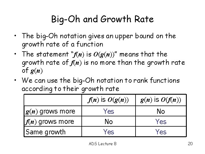
Big-Oh and Growth Rate • The big-Oh notation gives an upper bound on the growth rate of a function • The statement “f(n) is O(g(n))” means that the growth rate of f(n) is no more than the growth rate of g(n) • We can use the big-Oh notation to rank functions according to their growth rate g(n) grows more f(n) grows more Same growth f(n) is O(g(n)) g(n) is O(f(n)) Yes No Yes ADS Lecture 8 20