Chapter 32 The aggregate supply curve shows the

Chapter 32

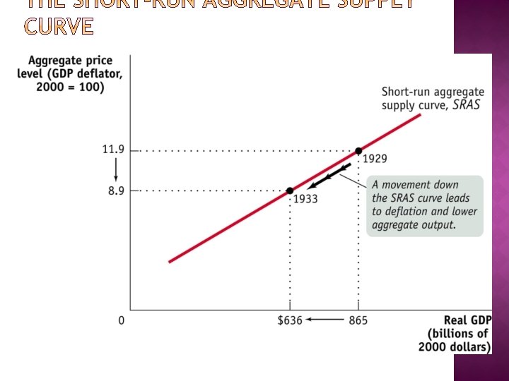
� The aggregate supply curve shows the relationship between the aggregate price level and the quantity of aggregate output in the economy. � GDP Deflator can be used as a measure of the price level �GDP Deflator= (Nom. GDP/Real GDP) *100 �An increasing GDP Deflator means an increasing price level

We generally think output prices change more quickly than input prices � The short-run aggregate supply curve is upwardsloping because nominal input prices, especially wages, are often “sticky” in the short run: � � a higher aggregate price level leads to higher profits (for a bit, at least) and increased aggregate output in the short run. The nominal wage is the dollar amount of the wage paid. � Sticky wages are nominal wages that are slow to fall even in the face of high unemployment and slow to rise even in the face of labor shortages. � Often other inputs are purchased under a contracted price as well and may be somewhat sticky �

� Producers supply goods based on their ability to make profits. � As opportunities for profits increase, they supply more.

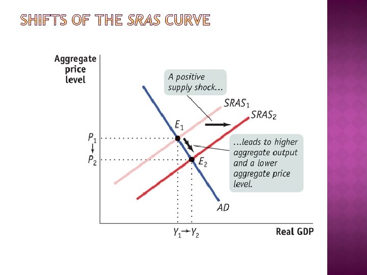
Changes in commodity prices If commodity prices fall, . . . short-run aggregate supply increases. If commodity prices rise, . . . short-run aggregate supply decreases. Changes in nominal wages If nominal wages fall, . . . short-run aggregate supply increases. If nominal wages rise, . . . short-run aggregate supply decreases. Changes in productivity If workers become more productive, . . . short-run aggregate supply increases. If workers become less productive, . . short-run aggregate supply decreases

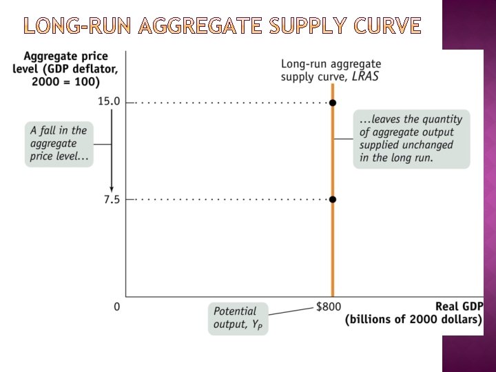
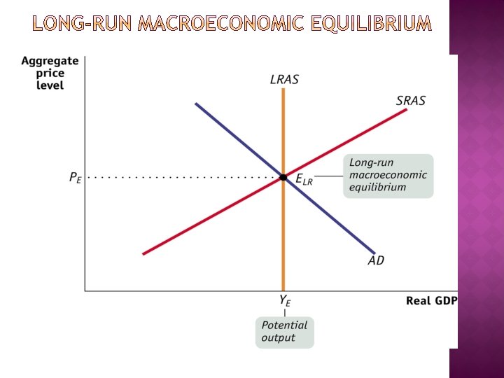
� The long-run aggregate supply curve shows the relationship between the aggregate price level and the quantity of aggregate output supplied that would exist if all prices, including nominal wages, were fully flexible. � While input prices, such as wages, probably are pretty sticky in the short-run, would they forever remain “stuck”? �No. Eventually existing contracts expire and new ones are negotiated. � In the LR, the aggregate price level has no effect on aggregate supply

� The LRAS curve represents the economy’s “potential output” or “potential GDP” � Potential Output: the level of real GDP the economy would produce if all prices (including wages) were instantly and perfectly flexible. �Think of this as the level of production, nationwide, that corresponds with full employment (and remember, full employment is not zero unemployment)

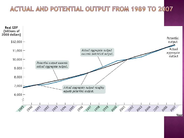
� While the economy’s actual output may not always be right at potential output, it will always fluctuate around it. �During recessions it will be slightly below, during expansions it will be slightly above.

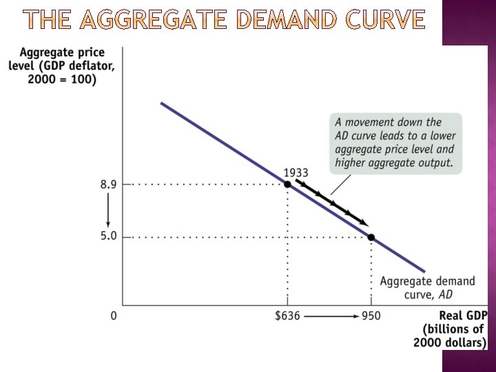
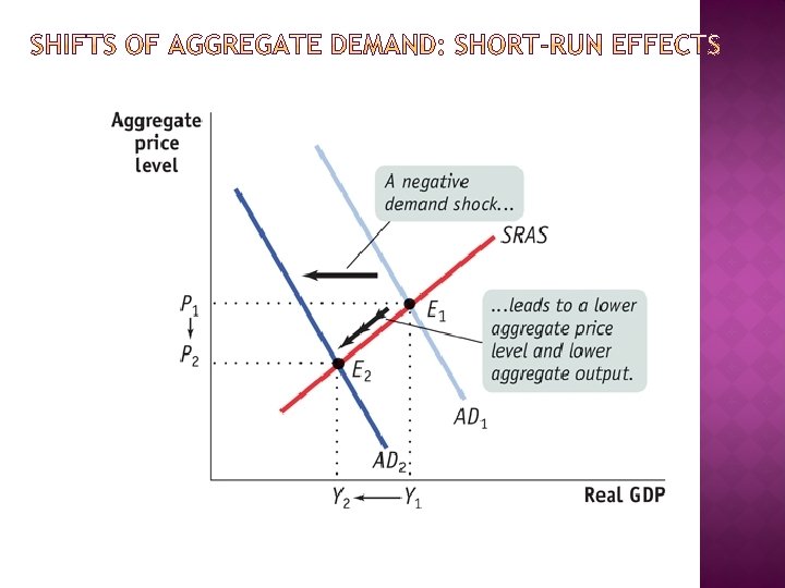
� The aggregate demand curve shows the relationship between the aggregate price level and the quantity of aggregate output demanded by households, businesses, the government and the rest of the world.

� It is downward-sloping for two reasons: �The first is the wealth effect of a change in the aggregate price level—a higher aggregate price level reduces the purchasing power of households’ wealth and reduces consumer spending. �The second is the interest rate effect of a change in aggregate price level—a higher aggregate price level reduces the purchasing power of households’ money holdings, leading to a rise in interest rates and a fall in investment spending and consumer spending.

� The aggregate demand curve shifts because of: �changes in expectations �wealth �the stock of physical capital �government policies fiscal policy monetary policy

Changes in expectations If consumers and firms become more optimistic, . . . aggregate demand increases. If consumers and firms become more pessimistic, . . . aggregate demand decreases. Changes in wealth If the real value of household assets rises, . . . aggregate demand increases. If the real value of household assets falls, . . . aggregate demand decreases. Fiscal policy If the government increases spending or cuts taxes, . . . aggregate demand increases. If the government reduces spending or raises taxes, . . aggregate demand decreases. Monetary policy If the central bank increases the quantity of money, . . . aggregate demand increases. If the central bank reduces the quantity of money, . . . aggregate demand decreases

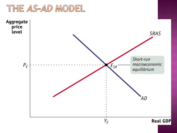
� The AS-AD model uses the aggregate supply curve and the aggregate demand curve together to analyze economic fluctuations.

� The economy is in short-run macroeconomic equilibrium when the quantity of aggregate output supplied is equal to the quantity demanded. � The short-run equilibrium aggregate price level is the aggregate price level in the short -run macroeconomic equilibrium. � Short-run equilibrium aggregate output is the quantity of aggregate output produced in the short-run macroeconomic equilibrium.

Stagflation is the combination of inflation and falling aggregate output.

� The economy is in long-run macroeconomic equilibrium when the point of short-run macroeconomic equilibrium is on the longrun aggregate supply curve.

Inflationary gap

Recessionary gap

� There is a recessionary gap when aggregate output is below potential output. � There is an inflationary gap when aggregate output is above potential output. � The output gap is the percentage difference between actual aggregate output and potential output.

� The economy is self-correcting when shocks to aggregate demand affect aggregate output in the short run, but not the long run. � Note that we think the economy will correct itself, given time. The problem is that this can takes years, sometimes perhaps even a decade. � Certain governmental policy (monetary policy and fiscal policy) can try to get us back in LR equilibrium faster. � This idea was championed by the British economist John Maynard Keynes, active during the Great Depression.

Supply Shocks versus Demand Shocks in Practice � Recessions are mainly caused by demand shocks. But when a negative supply shock does happen, the resulting recession tends to be particularly severe.

�Policy �There in the face of supply shocks: are no easy policies to shift the short-run aggregate supply curve. �Policy dilemma: a policy that counteracts the fall in aggregate output by increasing aggregate demand will lead to higher inflation, but a policy that counteracts inflation by reducing aggregate demand will deepen the output slump.

� Use the AS/AD model to analyze: � 1) An decrease in household optimism about the economy � 2) A stock market boom that increases household wealth � 3) The price of oil falls