Chapter 3 UTILITIES INDIFFERENCE CURVES Budget line 2

Chapter 3 UTILITIES INDIFFERENCE CURVES

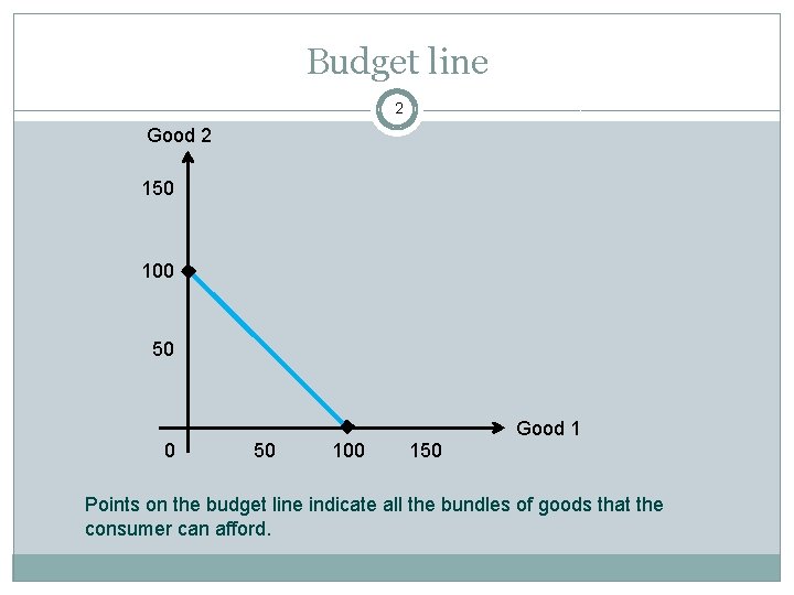
Budget line 2 Good 2 150 100 150 Good 1 Points on the budget line indicate all the bundles of goods that the consumer can afford.

Indifference Curve 3 �Indifference curve: locus of bundles that provide the consumer with the same level of satisfaction

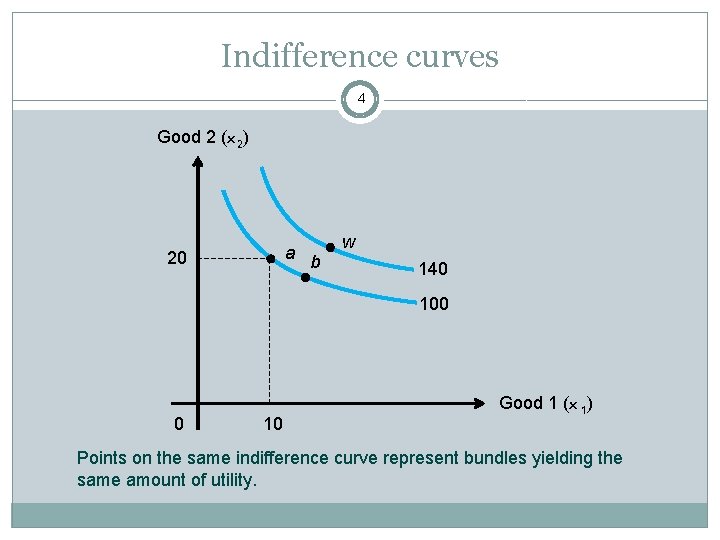
Indifference curves 4 Good 2 (x 2) a b 20 w 140 100 0 10 Good 1 (x 1) Points on the same indifference curve represent bundles yielding the same amount of utility.

Indifference Curves 5 �Indifference map Set of indifference curves for a consumer � Every bundle On an indifference curve Indifference curves � Farther from origin ->Higher utility

The Shape of Indifference Curves 6 �Indifference curves Cannot slope upward � Nonsatiation Cannot cross each other � Transitivity assumption and nonsatiation assumptions Farther from the origin – higher utility � Nonsatiation assumption � Cannot cross each other Are bowed in toward the origin � Convexity assumption � Farther from the origin - higher utility

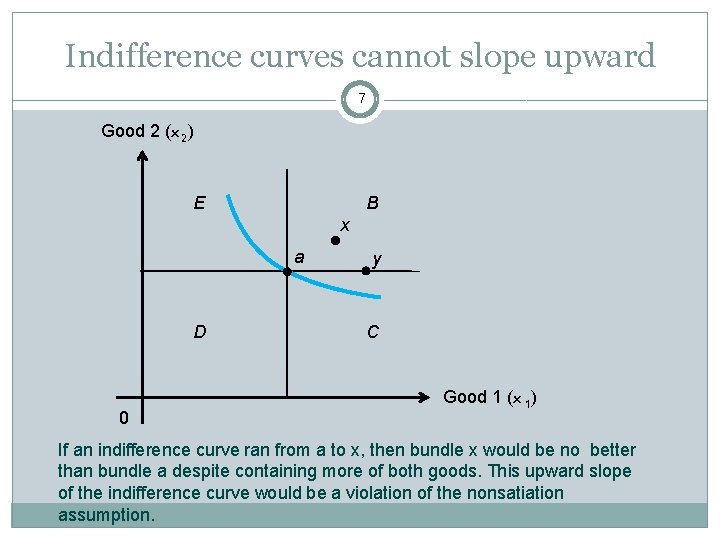
Indifference curves cannot slope upward 7 Good 2 (x 2) E B x a D 0 y C Good 1 (x 1) If an indifference curve ran from a to x, then bundle x would be no better than bundle a despite containing more of both goods. This upward slope of the indifference curve would be a violation of the nonsatiation assumption.

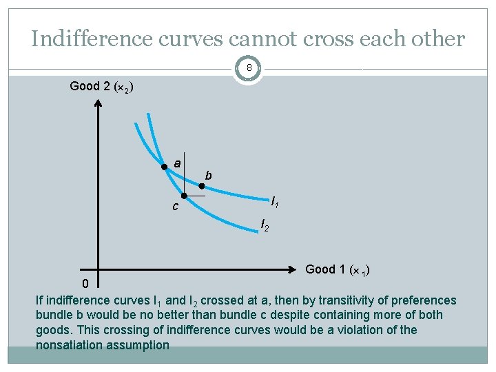
Indifference curves cannot cross each other 8 Good 2 (x 2) a b I 1 c I 2 Good 1 (x 1) 0 If indifference curves I 1 and I 2 crossed at a, then by transitivity of preferences bundle b would be no better than bundle c despite containing more of both goods. This crossing of indifference curves would be a violation of the nonsatiation assumption

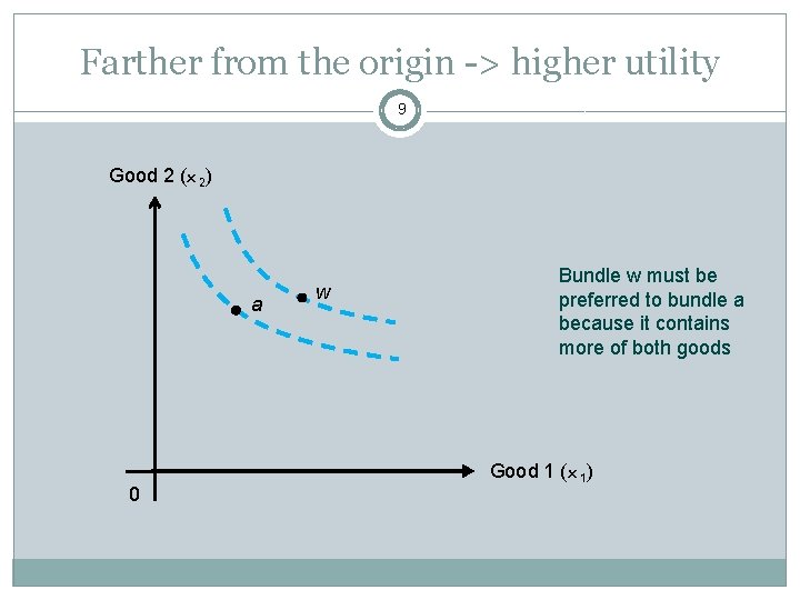
Farther from the origin -> higher utility 9 Good 2 (x 2) a 0 w Bundle w must be preferred to bundle a because it contains more of both goods Good 1 (x 1)

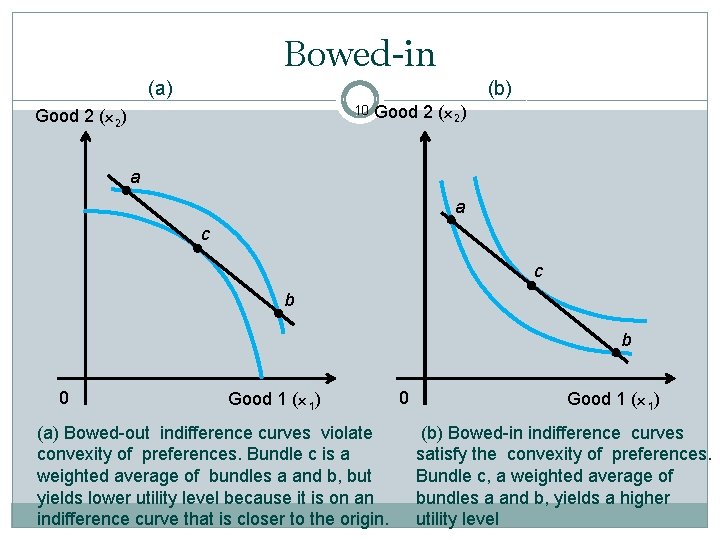
Bowed-in (b) (a) 10 Good 2 (x 2) a a c c b b 0 Good 1 (x 1) (a) Bowed-out indifference curves violate convexity of preferences. Bundle c is a weighted average of bundles a and b, but yields lower utility level because it is on an indifference curve that is closer to the origin. 0 Good 1 (x 1) (b) Bowed-in indifference curves satisfy the convexity of preferences. Bundle c, a weighted average of bundles a and b, yields a higher utility level

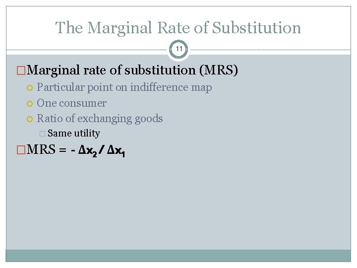
The Marginal Rate of Substitution 11 �Marginal rate of substitution (MRS) Particular point on indifference map One consumer Ratio of exchanging goods � Same utility �MRS = - ∆x 2 / ∆x 1

The Marginal Rate of Substitution 12 �Diminishing marginal rate of substitution From convexity Move along the indifference curve � Same utility level � MRS decreases

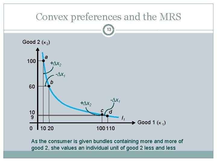
Convex preferences and the MRS 13 Good 2 (x 2) 100 a +∆x 2 -∆x 1 60 b -∆x 1 +∆x 2 c 10 9 0 10 20 d 100 110 I 1 Good 1 (x 1) As the consumer is given bundles containing more and more of good 2, she values an individual unit of good 2 less and less

Indifference Curves and Tastes 14 �Flat indifference curves Goods that yield no utility �Straight-line indifference curves Goods that are perfect substitutes � MRS - constant along an indifference curve � In a two-good world Indifference curve - straight line

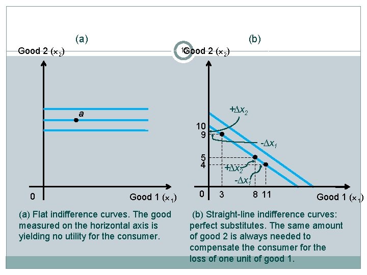
(b) (a) 15 Good 2 (x 2) +∆x 2 a 10 9 5 4 0 Good 1 (x 1) (a) Flat indifference curves. The good measured on the horizontal axis is yielding no utility for the consumer. 0 -∆x 1 +∆x 2 -∆x 1 3 8 11 Good 1 (x 1) (b) Straight-line indifference curves: perfect substitutes. The same amount of good 2 is always needed to compensate the consumer for the loss of one unit of good 1.

Indifference Curves and Tastes 16 �Right-angle indifference curves Goods that are perfect complements � Must be consumed in a fixed ratio to produce utility � In a two-good world Right angle indifference curves �Bowed-out indifference curves Nonconvex preferences

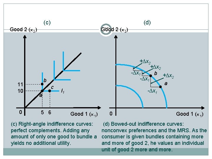
(d) (c) Good 2 (x 2) 11 10 0 17 Good 2 (x 2) +∆x 2 -∆x 1 b +∆x 2 -∆x 1 a -∆x 1 b c a 5 6 I 1 Good 1 (x 1) 0 Good 1 (x 1) (c) Right-angle indifference curves: (d) Bowed-out indifference curves: perfect complements. Adding any nonconvex preferences and the MRS. As the amount of only one good to bundle a consumer is given bundles containing more yields no additional utility. and more of good 2, he values an individual unit of good 2 more and more.

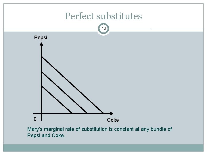
Perfect substitutes 18 Pepsi 0 Coke Mary’s marginal rate of substitution is constant at any bundle of Pepsi and Coke.

Optimal Consumption Bundle 19 �Optimal consumption bundle Maximize consumer’s utility � Within the economically feasible set Best bundle � According to consumer’s preferences �Characteristics of optimal bundles Indifference curve tangent to budget line Slope of indifference curve = MRS = -∆x 2/∆x 1 Slope of budget line = price ratio = p 1/p 2 � MRS = p 1/p 2

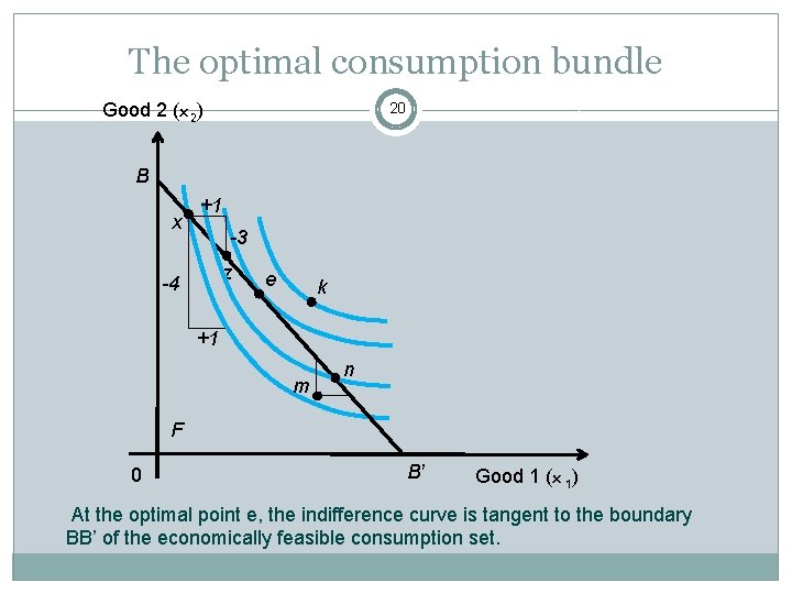
The optimal consumption bundle Good 2 (x 2) 20 B x +1 -3 z -4 e k +1 m n F 0 B’ Good 1 (x 1) At the optimal point e, the indifference curve is tangent to the boundary BB’ of the economically feasible consumption set.