Chapter 3 Using Spreadsheets in Analytical Chemistry Spreadsheet

Chapter 3: Using Spreadsheets in Analytical Chemistry

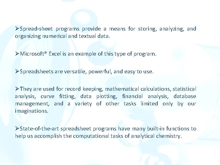
ØSpread-sheet programs provide a means for storing, analyzing, and organizing numerical and textual data. ØMicrosoft® Excel is an example of this type of program. ØSpreadsheets are versatile, powerful, and easy to use. ØThey are used for record keeping, mathematical calculations, statistical analysis, curve fitting, data plotting, financial analysis, database management, and a variety of other tasks limited only by our imaginations. ØState-of-the-art spreadsheet programs have many built-in functions to help us accomplish the computational tasks of analytical chemistry.

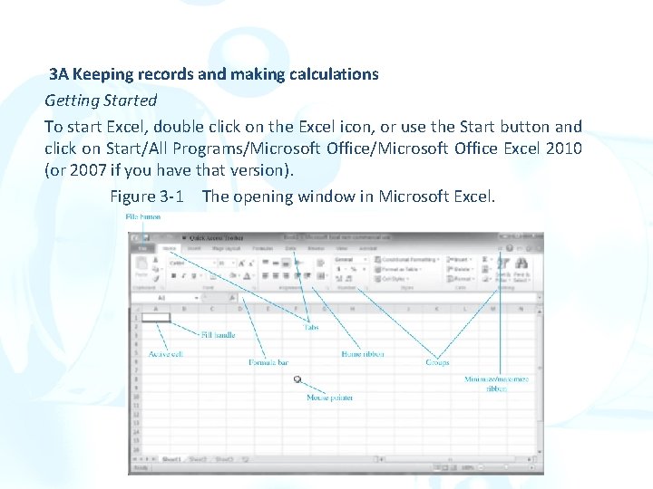
3 A Keeping records and making calculations Getting Started To start Excel, double click on the Excel icon, or use the Start button and click on Start/All Programs/Microsoft Office Excel 2010 (or 2007 if you have that version). Figure 3 -1 The opening window in Microsoft Excel.

1. Versions of Excel prior to Excel 2007 contained menus such as File, Edit, View, Insert, Format, and Tools, among others. 2. The menus and toolbars in Excel 2007 and 2010 are replaced by the ribbon, a two-dimensional layout of icons and words. 3. Each tab, such as Home, Insert, etc brings up a different ribbon with its own set of icons and descriptions. 4. It can be minimized by clicking the minimize ribbon arrow, by entering Ctrl 1 F 1, or by right clicking anywhere on the ribbon and selecting Minimize the Ribbon from the list that appears. 5. The worksheet consists of a grid of cells arranged in rows labeled 1, 2, 3, and so on, and columns labeled A, B, C, and so on. 6. Each cell has a unique location specified by its address.

1. The address of the active cell is always displayed in the box just above the first column of the displayed worksheet in the formula bar. 1. You can verify this display of the active cell by clicking on various cells of the work-sheet. 2. A workbook is a collection of worksheets and can be comprised of multiple worksheets available by clicking the tabs at the bottom labeled Sheet 1, Sheet 2, and so forth. 3. The term spreadsheet is a generic term and usually refers to a worksheet.

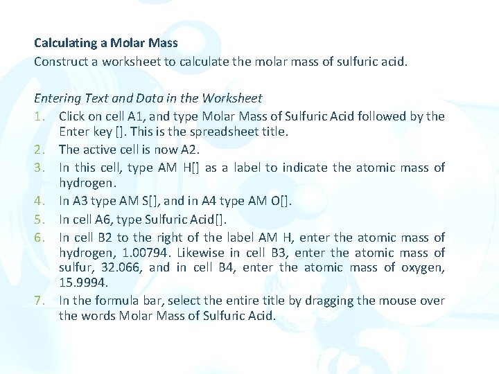
Calculating a Molar Mass Construct a worksheet to calculate the molar mass of sulfuric acid. Entering Text and Data in the Worksheet 1. Click on cell A 1, and type Molar Mass of Sulfuric Acid followed by the Enter key []. This is the spreadsheet title. 2. The active cell is now A 2. 3. In this cell, type AM H[] as a label to indicate the atomic mass of hydrogen. 4. In A 3 type AM S[], and in A 4 type AM O[]. 5. In cell A 6, type Sulfuric Acid[]. 6. In cell B 2 to the right of the label AM H, enter the atomic mass of hydrogen, 1. 00794. Likewise in cell B 3, enter the atomic mass of sulfur, 32. 066, and in cell B 4, enter the atomic mass of oxygen, 15. 9994. 7. In the formula bar, select the entire title by dragging the mouse over the words Molar Mass of Sulfuric Acid.

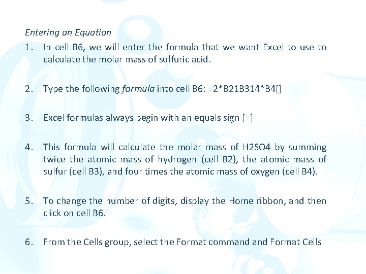
Entering an Equation 1. In cell B 6, we will enter the formula that we want Excel to use to calculate the molar mass of sulfuric acid. 2. Type the following formula into cell B 6: =2*B 21 B 314*B 4[] 3. Excel formulas always begin with an equals sign [=] 4. This formula will calculate the molar mass of H 2 SO 4 by summing twice the atomic mass of hydrogen (cell B 2), the atomic mass of sulfur (cell B 3), and four times the atomic mass of oxygen (cell B 4). 5. To change the number of digits, display the Home ribbon, and then click on cell B 6. 6. From the Cells group, select the Format command Format Cells

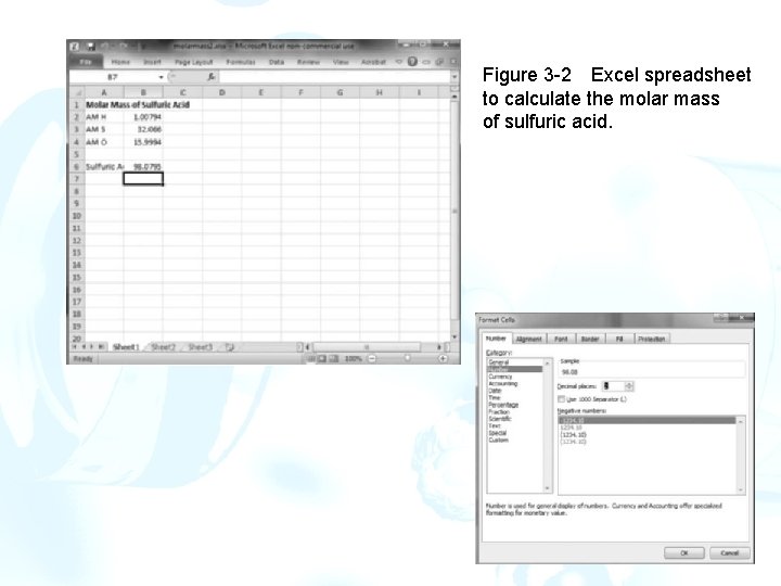
Figure 3 -2 Excel spreadsheet to calculate the molar mass of sulfuric acid.

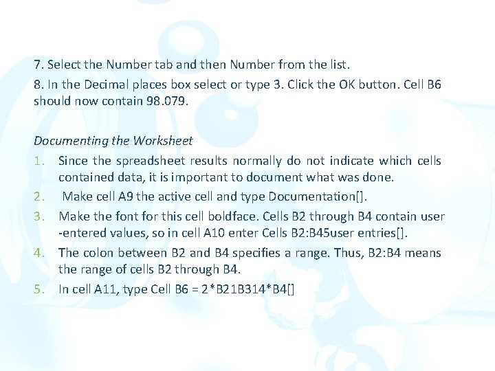
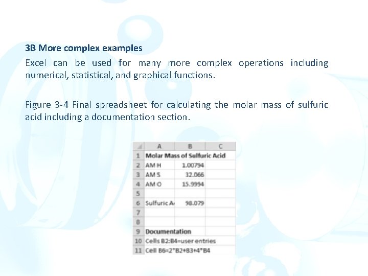
7. Select the Number tab and then Number from the list. 8. In the Decimal places box select or type 3. Click the OK button. Cell B 6 should now contain 98. 079. Documenting the Worksheet 1. Since the spreadsheet results normally do not indicate which cells contained data, it is important to document what was done. 2. Make cell A 9 the active cell and type Documentation[]. 3. Make the font for this cell boldface. Cells B 2 through B 4 contain user -entered values, so in cell A 10 enter Cells B 2: B 45 user entries[]. 4. The colon between B 2 and B 4 specifies a range. Thus, B 2: B 4 means the range of cells B 2 through B 4. 5. In cell A 11, type Cell B 6 = 2*B 21 B 314*B 4[]

All formulas in a worksheet can be revealed by holding the control key (Ctrl) while pressing and releasing the grave accent key ` located to the left of the number 1 key on the keyboard. Ø You can save the file to the hard disk by clicking on the File button and choosing Save As. ØYou can save as an Excel Workbook and various other formats including a format compatible with Excel 97 -2003. ØChoose Excel. Workbook and enter a location and a file name such as molar mass. ØExcel will automatically append the file extension. xlsx to the file name so that it will appear as molarmass. xlsx. ØChoosing to save in a format compatible with Excel 97 -2003 appends the file extension. xls to the file.

3 B More complex examples Excel can be used for many more complex operations including numerical, statistical, and graphical functions. Figure 3 -4 Final spreadsheet for calculating the molar mass of sulfuric acid including a documentation section.

A Laboratory Notebook Example Entering Text in the Worksheet Click on cell A 1, and as the worksheet title, type Gravimetric Determination of Chloride followed by the Enter key []. Continue to type text into the cells of column A. Mass of Bottle plus sample, g[ ] Mass of bottle less sample, g[ ] Mass of sample, g[ ] Crucible masses, with Ag. Cl, g[ ] Crucible masses, empty, g[ ] Mass of Ag. Cl, g[ ] %Chloride[ ]

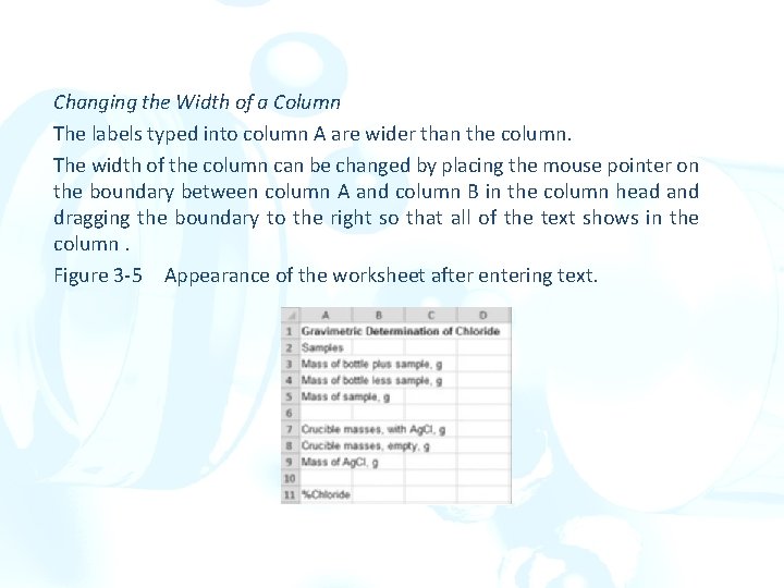
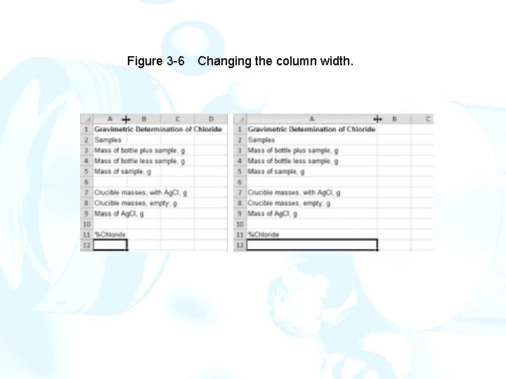
Changing the Width of a Column The labels typed into column A are wider than the column. The width of the column can be changed by placing the mouse pointer on the boundary between column A and column B in the column head and dragging the boundary to the right so that all of the text shows in the column. Figure 3 -5 Appearance of the worksheet after entering text.

Figure 3 -6 Changing the column width.

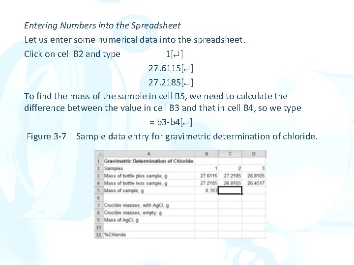
Entering Numbers into the Spreadsheet Let us enter some numerical data into the spreadsheet. Click on cell B 2 and type 1[ ] 27. 6115[ ] 27. 2185[ ] To find the mass of the sample in cell B 5, we need to calculate the difference between the value in cell B 3 and that in cell B 4, so we type = b 3 -b 4[ ] Figure 3 -7 Sample data entry for gravimetric determination of chloride.

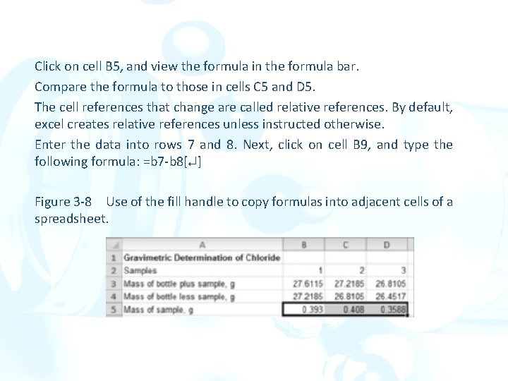
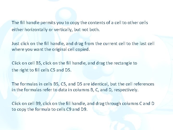
Filling Cells Using the Fill Handle The formulas for cells C 5 and D 5 are identical to the formula in cell B 5 except that the cell references for the data are different. In cell C 5, we want to compute the difference between the contents of cells C 3 and C 4, and in cell D 5, we want the difference between D 3 and D 4. To duplicate a formula in cells adjacent to an existing formula, simply click on the cell containing the formula (B 5 in our example), then click on the fill handle and drag the corner of the rectangle to the right so that it encompasses the cells where you want the formula to be duplicated.

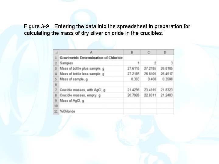
Click on cell B 5, and view the formula in the formula bar. Compare the formula to those in cells C 5 and D 5. The cell references that change are called relative references. By default, excel creates relative references unless instructed otherwise. Enter the data into rows 7 and 8. Next, click on cell B 9, and type the following formula: =b 7 -b 8[ ] Figure 3 -8 Use of the fill handle to copy formulas into adjacent cells of a spreadsheet.

Figure 3 -9 Entering the data into the spreadsheet in preparation for calculating the mass of dry silver chloride in the crucibles.

The fill handle permits you to copy the contents of a cell to other cells either horizontally or vertically, but not both. Just click on the fill handle, and drag from the current cell to the last cell where you want the original cell copied. Click on cell B 5, click on the fill handle, and drag the rectangle to the right to fill cells C 5 and D 5. The formulas in cells B 5, C 5, and D 5 are identical, but the cell references in the formulas refer to data in columns B, C, and D, respectively. Click on cell B 9, click on the fill handle, and drag through columns C and D to copy the formula to cells C 9 and D 9.

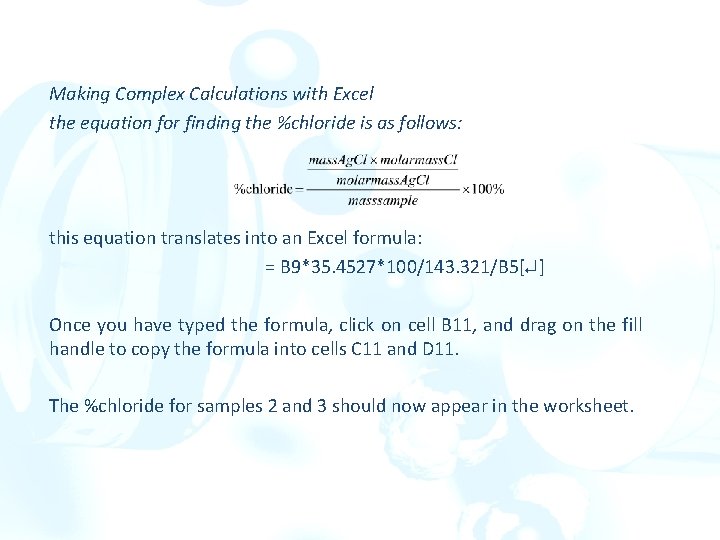
Making Complex Calculations with Excel the equation for finding the %chloride is as follows: this equation translates into an Excel formula: = B 9*35. 4527*100/143. 321/B 5[ ] Once you have typed the formula, click on cell B 11, and drag on the fill handle to copy the formula into cells C 11 and D 11. The %chloride for samples 2 and 3 should now appear in the worksheet.

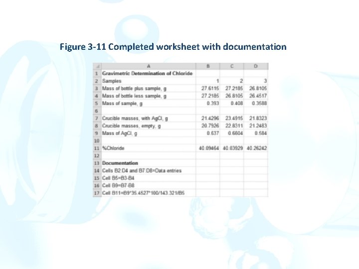
Documenting the Worksheet In cell A 13, type Documention[]. Cells B 2 through D 5 and B 7 through D 9 contain user-entered values. In cell A 14, enter Cells B 2: D 5 and B 7: D 95 Data entries[]. We now want to document the calculations done in cells B 5: D 5, B 9: D 9, and B 11: D 11. Figure 3 -10 Completing the calculation of percent chloride.

ØInstead of retyping the formulas, select cell A 15, and type Cell B 5[]. ØNow select cell B 5, and highlight the formula displayed in the formula bar. ØClick on the Copy icon in the Clipboard group on the Home tab as shown in the margin. ØTo prevent Excel from copying the formula and changing the cell references, hit the Escape key on the keyboard to cancel the operation. The text copied, however, is still in the Windows clipboard. ØSelect cell A 15, and position the cursor after the B 5 in the formula bar. ØClick on the Paste icon as shown in the margin. ØThis operation will copy the formula for the mass of sample into cell A 15 as a text string. ØBecause the same formula is used, the documentation does not need to include these cells. In cell A 16, type Cell B 9[]. Copy the formula from cell B 9 as before. ØIn Cell A 17, type Cell B 11[], and copy the formula from this cell.

Figure 3 -11 Completed worksheet with documentation

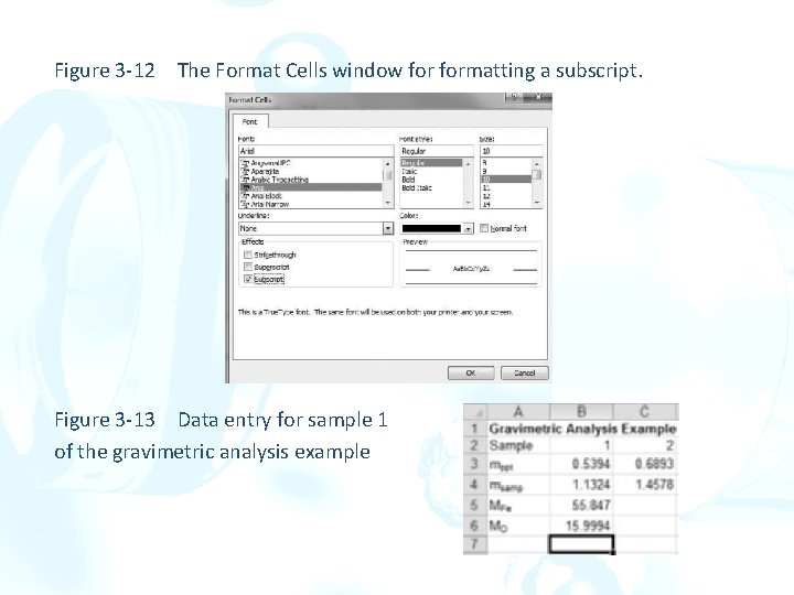
Another Example from Gravimetric Analysis Compute the percentage of Fe and Fe 3 O 4 in two samples of an iron ore. The samples were precipitated as Fe 2 O 3∙x. H 2 O, and the residue was ignited to give pure Fe 2 O 3. More Cell Formatting ØSelect cell A 1, and type a title such as Gravimetric Analysis Example. ØIn cell A 2, type Sample and put the sample numbers in cell B 2 and C 2. ØIn cell A 3, type mppt. ØTo make the abbreviation ppt appear as a subscript as in mppt. Select cell A 3. In the formula bar, use the mouse to highlight (select) the ppt part of mppt. Click the right mouse button, and select Format Cells from the list. ØFormat Cells window contains tabs for Number, Alignment, Font, Border, Fill, and Protection. ØSelect Subscript in the Effects box so that a checkmark appears. Click on the OK button, and note that cell A 2 now contains mppt as a label for mass of precipitate.

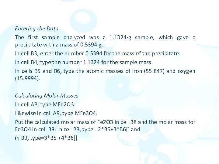
Entering the Data The first sample analyzed was a 1. 1324 -g sample, which gave a precipitate with a mass of 0. 5394 g. In cell B 3, enter the number 0. 5394 for the mass of the precipitate. In cell B 4, type the number 1. 1324 for the sample mass. In cells B 5 and B 6, type the atomic masses of iron (55. 847) and oxygen (15. 9994). Calculating Molar Masses In cell A 8, type MFe 2 O 3. Likewise in cell A 9, type MFe 3 O 4. Put the calculated molar mass of Fe 2 O 3 in cell B 8 and the molar mass for Fe 3 O 4 in cell B 9. In cell B 8, type =2*B 5+3*B 6[] and in B 9, type=3*B 5 +4*B 6[]

Figure 3 -12 The Format Cells window formatting a subscript. Figure 3 -13 Data entry for sample 1 of the gravimetric analysis example

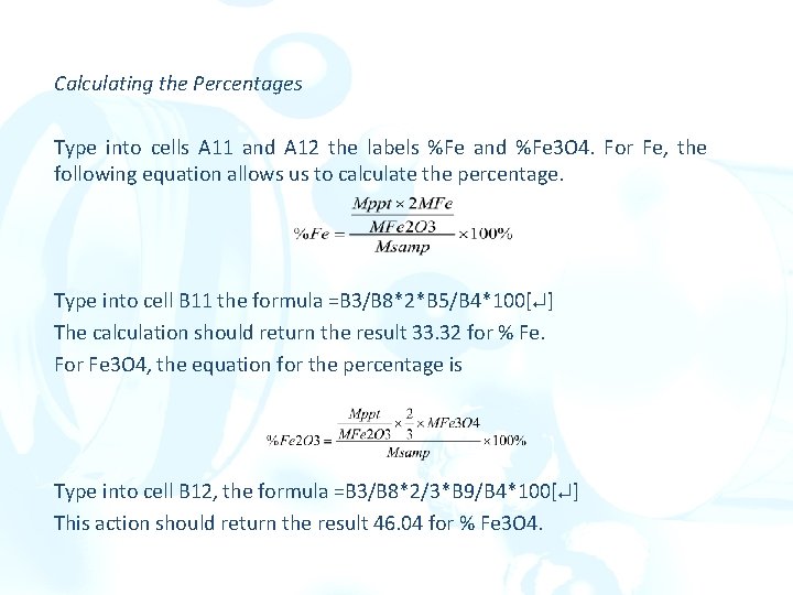
Calculating the Percentages Type into cells A 11 and A 12 the labels %Fe and %Fe 3 O 4. For Fe, the following equation allows us to calculate the percentage. Type into cell B 11 the formula =B 3/B 8*2*B 5/B 4*100[ ] The calculation should return the result 33. 32 for % Fe. For Fe 3 O 4, the equation for the percentage is Type into cell B 12, the formula =B 3/B 8*2/3*B 9/B 4*100[ ] This action should return the result 46. 04 for % Fe 3 O 4.

Finding the Percentages for Sample 2: Using Absolute References For Sample 2, a sample mass of 1. 4578 g gave a precipitate mass of 0. 6893 g. Enter these values into cells C 3 and C 4. Use the same atomic mass for Fe in cell B 5 and the same molar masses for Fe 2 O 3 and Fe 3 O 4 in cells B 8 and B 9. We can make a reference an absolute reference by putting a dollar sign before the column letter and a second dollar sign before the row number. With the cursor on cell A 1, click on Find & Select on the Home ribbon. Choose Replace… from the drop-down menu. Enter B 5 in the Find box and $B$5 in the Replace

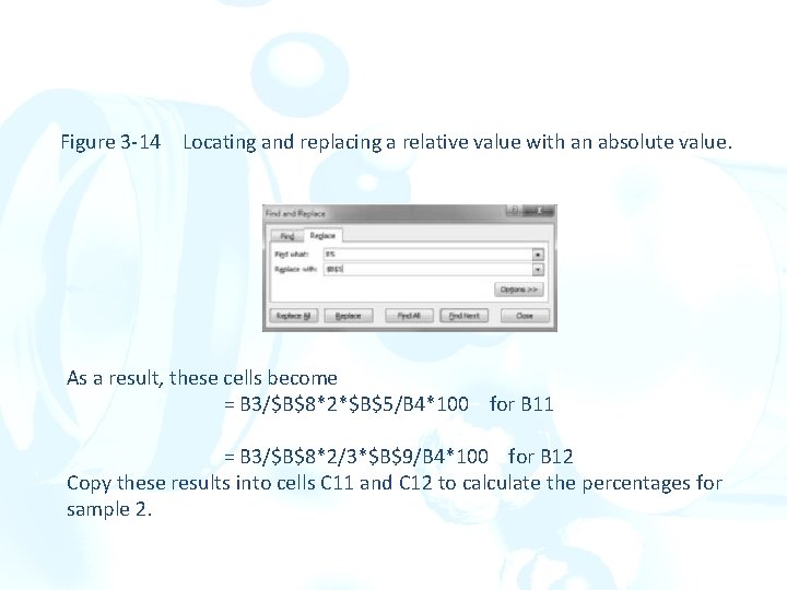
Figure 3 -14 Locating and replacing a relative value with an absolute value. As a result, these cells become = B 3/$B$8*2*$B$5/B 4*100 for B 11 = B 3/$B$8*2/3*$B$9/B 4*100 for B 12 Copy these results into cells C 11 and C 12 to calculate the percentages for sample 2.

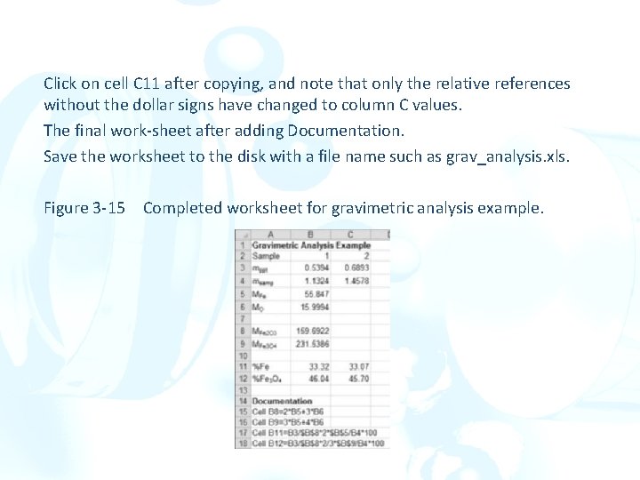
Click on cell C 11 after copying, and note that only the relative references without the dollar signs have changed to column C values. The final work-sheet after adding Documentation. Save the worksheet to the disk with a file name such as grav_analysis. xls. Figure 3 -15 Completed worksheet for gravimetric analysis example.