Chapter 3 UNCONSTRAINED OPTIMIZATION Prof S S Jang

Chapter 3 UNCONSTRAINED OPTIMIZATION Prof. S. S. Jang Department of Chemical Engineering National Tsing-Hua Univeristy

Contents l Optimality Criteria l Direct Search Methods • • • Nelder and Mead (Simplex Search) Hook and Jeeves(Pattern Search) Powell’s Method (The Conjugated Direction Search) l Gradient Based Methods • • Cauchy’s method (the Steepest Decent) Newton’s Method Conjugate Gradient Method (The Fletcher and Reese Method) Quasi-Newton Method – Variable Metric Method

3 -1 The Optimality Criteria l Given a function (objective function) f(x), where and let ¡ Stationary Condition: ¡ Sufficient minimum criteria positive definite ¡ Sufficient maximum criteria negative definite

Definiteness l A real quadratic for Q=x. TCx and its symmetric matrix C=[cjk] are said to be positive definite (p. d. ) if Q>0 for all x≠ 0. A necessary and sufficient condition for p. d. is that all the determinants: are positive, C is negative definitive (n. d. ) if –C is p. d.

Example : l x=linspace(-3, 3); y=x; l >> for i=1: 100 l for j=1: 100 l z(i, j)=2*x(i)+4*x(i)*y(j)-10*x(i)*y(j)^3+y(j)^2; l end l mesh(x, y, z) l contour(x, y, z, 100)

Example- Continued (mesh and contour)

Example-Continued At Indefinite, x* is a non-optimum point.

Mesh and Contour – Himmelblau’s function : f(x)=(x 12+x 2 -11)2+(x 1+x 22 -7)2 l Optimality Criteria may find a local minimum in this case lx=linspace(-5, 5); y=x; l for i=1: 100 lfor j=1: 100 lz(i, j)=(x(i)^2+y(j)-11)^2+(x(i)+y(j)^2 -7)^2; lend lmesh(x, y, z) lcontour(x, y, z, 80)

Mesh and Contour - Continued

Example: f(x)=x 12+25 x 22

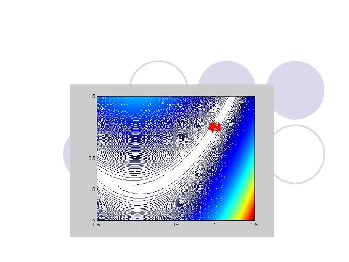
Rosenbrock’s Banana Function f(x, y)=100(y-x 2)2+(1 -x)2

Example: f(x)=2 x 13+4 x 1 x 23 -10 x 1 x 2+x 23 Steepest decent search from the initial point at (2, 2); we have d=[6 x 12+4 x 23 -10 x 2, 12 x 1 x 22 -10 x 1+3 x 22]’=

Example: Curve Fitting l From theoretical considerations, it is believe that the dependent variable y is related to variable x via a two-parameter function: The parameters k 1 and k 2 are to be determined by a least square of the following experimental data: x y 1. 0 2. 0 3. 0 4. 0 1. 05 1. 25 1. 59

Problem Formulation and mesh, contour

The Importance of One-dimensional Problem - The Iterative Optimization Procedure Consider a objective function Min f(X)= x 12+x 22, with an initial point X 0=(-4, -1) and a direction (1, 0), what is the optimum at this direction, i. e. X 1=X 0 + *(1, 0). This is a one -dimensional search for .

3 -2 Steepest Decent Approach – Cauchy’s Method l A direction d=[x 1, x 2, . . , xn]’ is a ndimensional vector, a line search is an approach such that from a based point x 0, find *, for all , x 0+ *d is an optimum. l Theorem: the direction d=-[ f/ x 1, f/ x 2, . . , f/ xn]’ is the steepest decent direction. Proof: Consider a two dimensional system: f(x 1, x 2), the movement ds 2=dx 12+dx 22, and f= ( f/ x 1)dx 1+ ( f/ x 2)dx 2= ( f/ x 1)dx 1+ ( f/ x 2)(ds 2 -dx 12)1/2. Then to maximize the change f, we have d( f)/dx 1=0. It can be shown that dx 1/ds= ( f/ x 1)/( ( f/ x 1)2 + ( f/ x 2)2)1/2, dx 2/ds= ( f/ x 2)/( ( f/ x 1)2+ ( f/ x 2)2)1/2

Example: f(x)=2 x 13+4 x 1 x 23 -10 x 1 x 2+x 23 Steepest decent search from the initial point at (2, 2); we have d=[6 x 12+4 x 23 -10 x 2, 12 x 1 x 22 -10 x 1+3 x 22]’=

Quadratic Function Properties Property #1: Optimal linear search for a quadratic function:

Quadratic Function Properties- Continued Property #2 fk+1 is orthogonal to sk for a quadratic function

3 -2 Newton’s Method – Best Convergence approaching the optimum

3 -2 Newton’s Method – Best Convergence approaching the optimum

Comparison of Newton’s Method and Cauchy’s Method

Remarks l Newton’s method is much more efficient than Steep Decent approach. Especially, the starting point is getting close to the optimum. l There is a requirement for the positive definite of the hessian in implementing Newton’s method. Otherwise, the search will be diverse. l The evaluation of hessian requires second derivative of the objective function, thus, the number of function evaluation will be drastically increased if a numerical derivative is used. l Steepest decent is very inefficient around the optimum, but very efficient at the very beginning of the search.

Conclusion l Cauchy’s method is very seldom to use because of its inefficiency around the optimum. l Newton’s method is also very seldom to use because of the requirement of second derivative. l A useful approach should be somewhere in between.

3 -3 Method of Powell’s Conjugate Direction l Definition: Let u and v denote two vectors in En. They are said to be orthogonal, if their scalar product equals to zero, i. e. u v=0. Similarly, u and v are said to be mutually conjugative with respect to a matrix A, if u and Av are mutually orthogonal, i. e. u Av=0. l Theorem: If conjugate directions to the hessian are used to any quadratic function of n variables that has a minimum, can be minimized in n steps.

Powell’s Conjugated Direction Method. Continued l Corollary: Generation of conjugated vectors. Extended Parallel Space Property ¡ Given a direction d and two initial point x(1), x(2), we assume:

Powell’s Algorithm l Step 1: Define x 0, and set N linearly indep. Directions say: l s(i)=e(i) l Step 2: Perfrom N+1 one directional searches along with s(N), s(1), , s(N) l Step 3: Form the conjugate direction d using the extended parallel space property. l Step 4: Set l Go to Step 2

Powell’s Algorithm (MATLAB) l l l l l l l l l l function opt=powell_n_dim(x 0, n, eps, tol, opt_func) xx=x 0; obj_old=feval(opt_func, x 0); s=zeros(n, n); obj=obj_old; df=100; absdx=100; for i=1: n; s(i, i)=1; end while df>eps/absdx>tol x_old=xx; for i=1: n+1 if(i==n+1) j=1; else j=i; end ss=s(: , j); alopt=one_dim_pw(xx, ss', opt_func); xx=xx+alopt*ss'; if(i==1) y 1=xx; end if(i==n+1) y 2=xx; end d=y 2 -y 1; nn=norm(d, 'fro'); for i=1: n d(i)=d(i)/nn; end dd=d'; alopt=one_dim_pw(xx, dd', opt_func); xx=xx+alopt*d dx=xx-x_old; plot(xx(1), xx(2), 'ro') absdx=norm(dx, 'fro'); obj=feval(opt_func, xx); df=abs(obj-obj_old); obj_old=obj; for i=1: n-1 s(: , i)=s(: , i+1); end s(: , n)=dd; end opt=xx

Example: f(x)=x 12+25 x 22

Example 2: Rosenbrock’s function

Example: fittings l x 0=[3 3]; opt=fminsearch('fittings', x 0) l opt = l 2. 0884 1. 0623

Fittings

Function Fminsearch l >> help fminsearch l l l l l l l l l l l FMINSEARCH Multidimensional unconstrained nonlinear minimization (Nelder-Mead). X = FMINSEARCH(FUN, X 0) starts at X 0 and finds a local minimizer X of the function FUN accepts input X and returns a scalar function value F evaluated at X. X 0 can be a scalar, vector or matrix. X = FMINSEARCH(FUN, X 0, OPTIONS) minimizes with the default optimization parameters replaced by values in the structure OPTIONS, created with the OPTIMSET function. See OPTIMSET for details. FMINSEARCH uses these options: Display, Tol. X, Tol. Fun, Max. Fun. Evals, and Max. Iter. X = FMINSEARCH(FUN, X 0, OPTIONS, P 1, P 2, . . . ) provides for additional arguments which are passed to the objective function, F=feval(FUN, X, P 1, P 2, . . . ). Pass an empty matrix for OPTIONS to use the default values. (Use OPTIONS = [] as a place holder if no options are set. ) [X, FVAL]= FMINSEARCH(. . . ) returns the value of the objective function, described in FUN, at X. [X, FVAL, EXITFLAG] = FMINSEARCH(. . . ) returns a string EXITFLAG that describes the exit condition of FMINSEARCH. If EXITFLAG is: 1 then FMINSEARCH converged with a solution X. 0 then the maximum number of iterations was reached. [X, FVAL, EXITFLAG, OUTPUT] = FMINSEARCH(. . . ) returns a structure OUTPUT with the number of iterations taken in OUTPUT. iterations. Examples FUN can be specified using @: X = fminsearch(@sin, 3) finds a minimum of the SIN function near 3. In this case, SIN is a function that returns a scalar function value SIN evaluated at X. FUN can also be an inline object: X = fminsearch(inline('norm(x)'), [1; 2; 3]) returns a minimum near [0; 0; 0]. FMINSEARCH uses the Nelder-Mead simplex (direct search) method. See also OPTIMSET, FMINBND, @, INLINE.

Pipeline design P 2 P 1 … L D Q

3 -4 Conjugated Gradient Method Fletcher-Reeves’s Method (FRP) l Given s 1=- f 1, s 2=- f 2+ s 1 l It can be shown that if l where, s 2 is started at the optimum of the line search along the direction s 1. And f a+b. Txk+1/2 xk. THxk, then s 2 is conjugated to s 1 with respect to H l Most general iteration:

Example: (The Fletcher-Reeves Method for Rosenbrock’s function )

3 -5 Quasi-Newton’s Method (Variable Matrix Method) l The variable matric approach is using an approximate Hessian matrix without taking second derivative of the objective function, the Newton’s direction can be approximated by: xk+1=xk- k. Ak fk l As Ak=I Cauchy’s direction l As Ak=H-1 Newton’s direction l In the variable matric approach, Ak can be updated to approximate the inverse of the Hessian by iterative approaches

3 -5 Quasi-Newton’s Method (Variable Matrix Method)- Continued l Given the objective function f(x) a+bx+ 1/2 x. THx, then f b+Hx, and fk+1 - f k H(xk+1 - xk ), or xk+1 - xk= H-1 gk where gk = fk+1 - f k l Let Ak+1=H-1 = Ak+ Ak xk+1 - xk= (Ak+ Ak ) gk l Ak gk = xk- Ak gk l Finally,

Quasi-Newton’s Method – Continued l Choose y= xk, z= Ak gk (The Davidon-Flecher-Powell’s method l Broyden-Flecher-Shanno’s Method l Summary: l In the first run, given initial conditions and convergence criteria, and evaluate the gradient l First direction is on the negative of the gradient, Ak =I l In the iteration phase, evaluate the new gradient and find gk, xk, and solve Ak using the equation in the previous slide l The new direction is on sk+1=Ak+1 f k+1 l Check convergence, and continue the iteration phase

Example: (The BFS Method for Rosenbrock’s function )

Heuristic Approaches (1) s-2 Simplex Approach l Main Idea Trial Point Base Point l Rules l 1: Straddled: Selected the “worse” vertex generated in the previous iteration, then choose instead the vertex with the next highest function value l 2. Cycling: In a given vertex unchanged more than M iterations, reduce the size by some factor l 3. Termination: The search is terminated when the simlex gets small enough.

Example: Rosenbrock Function

Simplex Approach: Nelder and Mead xnew z xnew xc X(h) xnew X(h) xc xnew X(h) z xc z X(h) xc

Comparisons of Different Approach for Solving Rosenbrock function Method subprogram Optimum found Number of iterations Cost function value Number of function called Cauchy’s Steepest_decent_ rosenbrock 0. 9809 0. 9622 537 3. 6379 e-004 11021 Newton’s Newton_method_rosenbroc k 0. 9993 0. 9985 9 1. 8443 e-006 N/A Powell’s Pw_rosenbrock_main 1. 0000 0. 9999 10 3. 7942 e-009 799 Fletcher. Reeves Frp_rosenbrock_main 0. 9906 0. 9813 8 8. 7997 e-005 155 Broyden_Fletc her_Shanno Bfs_rosenbrock_main 1. 0000 1. 0001 17 1. 0128 e-004 388 Nelder/Mead fminsearch 1. 0000 N/A 3. 7222 e-010 103

Heuristic Approach (Reduction Sampling with Random Search) l Step 1: Given initial sampling radius and initial center of the generate a random N points within the region. l Step 2: Get the best of the N sampling as the new center of the circle. l Step 3: Reduce the radius of the search circle, if the radius is not small enough, go back to step 2, otherwise stop.