Chapter 3 The simplex algorithm Putting Linear Programs
- Slides: 46

Chapter 3. The simplex algorithm Putting Linear Programs into standard form l Introduction to Simplex Algorithm l from a presentation at the Fuqua School of Business MIT and James Orlin © 2003 Rev. 3. 1 by M. Miccio on December 17, 2014 file Simplex 2_AMII_05 a_gr MIT and James Orlin © 2003 1

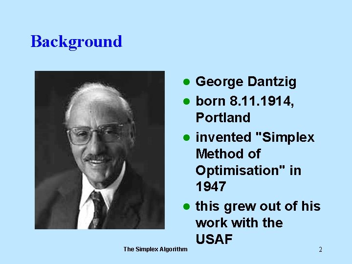
Background George Dantzig l born 8. 11. 1914, Portland l invented "Simplex Method of Optimisation" in 1947 l this grew out of his work with the USAF l The Simplex Algorithm 2

Background l originates from military planning tasks: – plans or schedules for training – logistical supply – deployment of men l has usually a “polynomial” computational cost The Simplex Algorithm 3

Overview of Lecture l l l Getting an LP into standard form Getting an LP into canonical form Optimality conditions Improving a solution A simplex pivoting MIT and James Orlin © 2003 4

Overview of Lecture l Getting an LP into standard form MIT and James Orlin © 2003 5

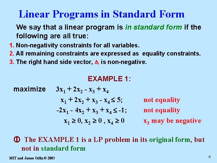
Linear Programs in Standard Form We say that a linear program is in standard form if the following are all true: 1. Non-negativity constraints for all variables. 2. All remaining constraints are expressed as equality constraints. 3. The right hand side vector, b, is non-negative. maximize EXAMPLE 1: 3 x 1 + 2 x 2 - x 3 + x 4 x 1 + 2 x 2 + x 3 - x 4 5; -2 x 1 - 4 x 2 + x 3 + x 4 -1; x 1 0, x 2 0 , x 4 0 not equality x 3 may be negative The EXAMPLE 1 is a LP problem in its original form, but not in standard form MIT and James Orlin © 2003 6

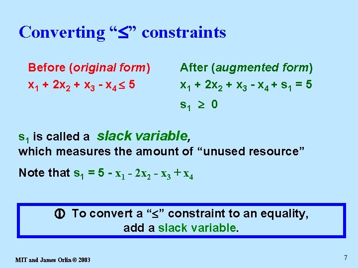
Converting “ ” constraints Before (original form) x 1 + 2 x 2 + x 3 - x 4 5 After (augmented form) x 1 + 2 x 2 + x 3 - x 4 + s 1 = 5 s 1 0 s 1 is called a slack variable, which measures the amount of “unused resource” Note that s 1 = 5 - x 1 - 2 x 2 - x 3 + x 4 To convert a “ ” constraint to an equality, add a slack variable. MIT and James Orlin © 2003 7

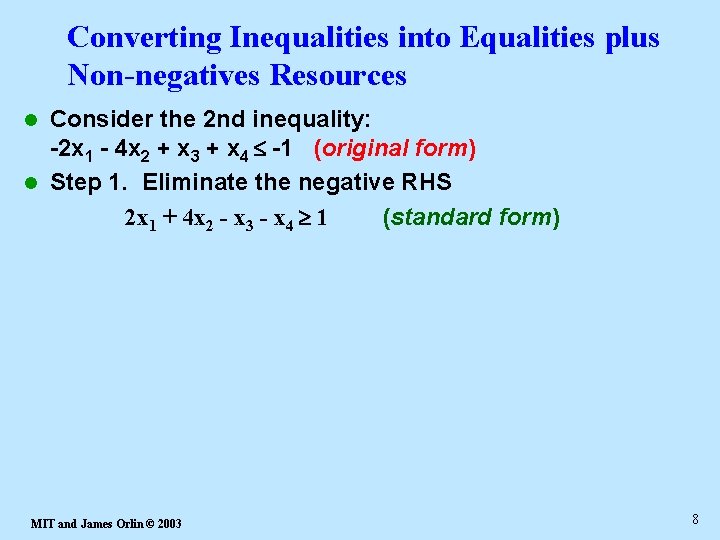
Converting Inequalities into Equalities plus Non-negatives Resources Consider the 2 nd inequality: -2 x 1 - 4 x 2 + x 3 + x 4 -1 (original form) l Step 1. Eliminate the negative RHS 2 x 1 + 4 x 2 - x 3 - x 4 1 (standard form) l MIT and James Orlin © 2003 8

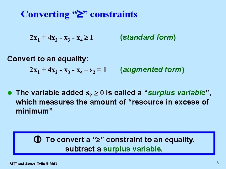
Converting “ ” constraints 2 x 1 + 4 x 2 - x 3 - x 4 1 Convert to an equality: 2 x 1 + 4 x 2 - x 3 - x 4 – s 2 = 1 l (standard form) (augmented form) The variable added s 2 0 is called a “surplus variable”, which measures the amount of “resource in excess of minimum” To convert a “ ” constraint to an equality, subtract a surplus variable. MIT and James Orlin © 2003 9

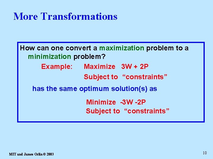
More Transformations How can one convert a maximization problem to a minimization problem? Example: Maximize 3 W + 2 P Subject to “constraints” has the same optimum solution(s) as Minimize -3 W -2 P Subject to “constraints” MIT and James Orlin © 2003 10

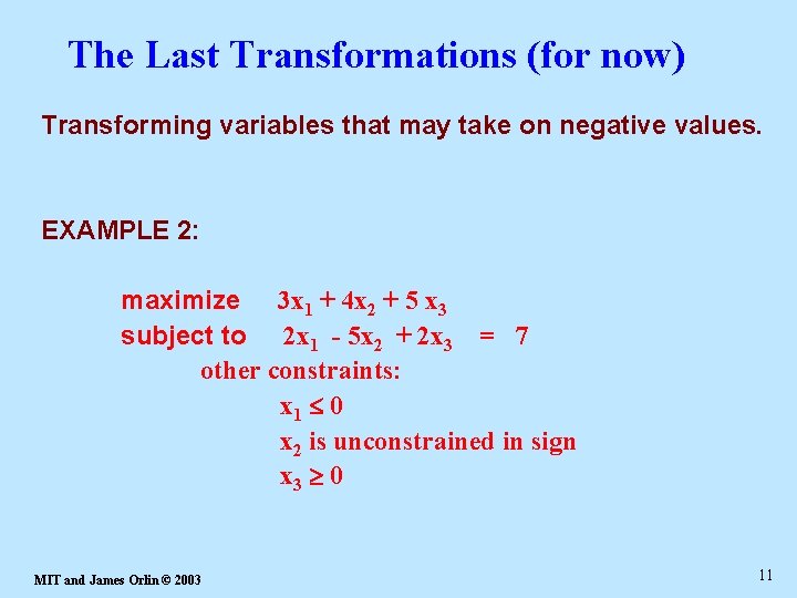
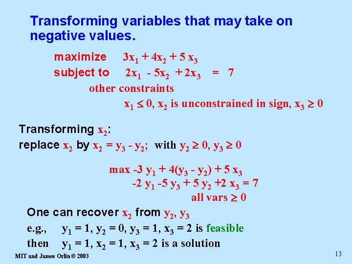
The Last Transformations (for now) Transforming variables that may take on negative values. EXAMPLE 2: maximize 3 x 1 + 4 x 2 + 5 x 3 subject to 2 x 1 - 5 x 2 + 2 x 3 = 7 other constraints: x 1 0 x 2 is unconstrained in sign x 3 0 MIT and James Orlin © 2003 11

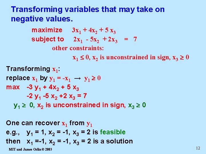
Transforming variables that may take on negative values. maximize 3 x 1 + 4 x 2 + 5 x 3 subject to 2 x 1 - 5 x 2 + 2 x 3 = 7 other constraints: x 1 0, x 2 is unconstrained in sign, x 3 0 Transforming x 1: replace x 1 by y 1 = -x 1 → y 1 0 max -3 y 1 + 4 x 2 + 5 x 3 -2 y 1 -5 x 2 +2 x 3 = 7 y 1 0, x 2 is unconstrained in sign, x 3 0 One can recover x 1 from y 1 e. g. , y 1 = 1, x 2 = -1, x 3 = 2 is feasible then x 1 =-1, x 2 = -1, x 3 = 2 is a solution MIT and James Orlin © 2003 12

Transforming variables that may take on negative values. maximize 3 x 1 + 4 x 2 + 5 x 3 subject to 2 x 1 - 5 x 2 + 2 x 3 = 7 other constraints x 1 0, x 2 is unconstrained in sign, x 3 0 Transforming x 2: replace x 2 by x 2 = y 3 - y 2; with y 2 0, y 3 0 max -3 y 1 + 4(y 3 - y 2) + 5 x 3 -2 y 1 -5 y 3 + 5 y 2 +2 x 3 = 7 all vars 0 One can recover x 2 from y 2, y 3 e. g. , y 1 = 1, y 2 = 0, y 3 = 1, x 3 = 2 is feasible then y 1 = 1, x 2 = 1, x 3 = 2 is a solution MIT and James Orlin © 2003 13

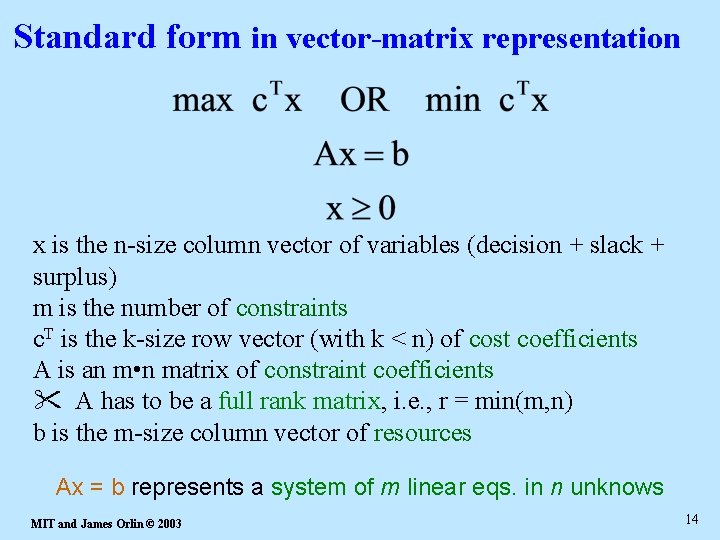
Standard form in vector-matrix representation x is the n-size column vector of variables (decision + slack + surplus) m is the number of constraints c. T is the k-size row vector (with k < n) of cost coefficients A is an m • n matrix of constraint coefficients A has to be a full rank matrix, i. e. , r = min(m, n) b is the m-size column vector of resources Ax = b represents a system of m linear eqs. in n unknows MIT and James Orlin © 2003 14

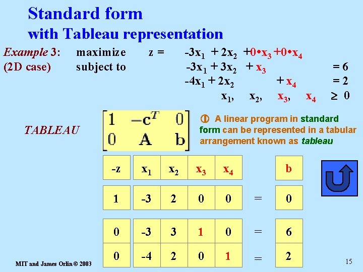
Standard form with Tableau representation Example 3: (2 D case) maximize subject to z= -3 x 1 + 2 x 2 +0 x 3 +0 x 4 -3 x 1 + 3 x 2 + x 3 -4 x 1 + 2 x 2 + x 4 x 1, x 2, x 3, x 4 A linear program in standard TABLEAU MIT and James Orlin © 2003 =6 =2 0 form can be represented in a tabular arrangement known as tableau -z x 1 x 2 x 3 x 4 1 -3 2 0 0 = 0 0 -3 3 1 0 = 6 0 -4 2 0 1 = 2 b 15

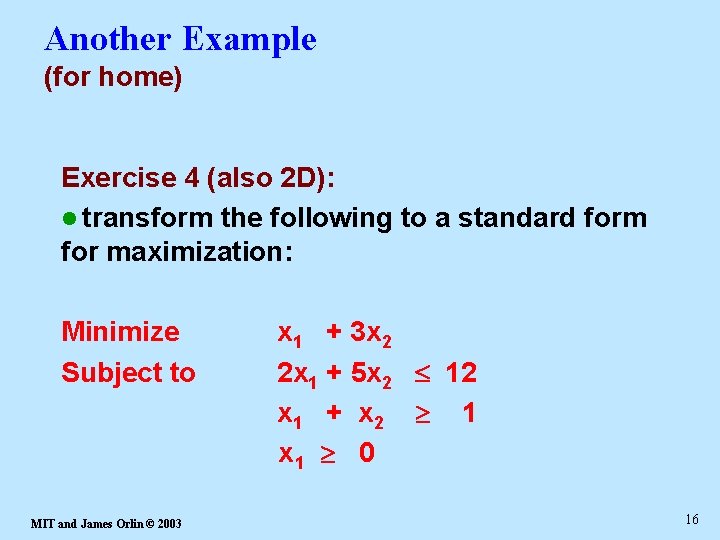
Another Example (for home) Exercise 4 (also 2 D): l transform the following to a standard form for maximization: Minimize Subject to MIT and James Orlin © 2003 x 1 + 3 x 2 2 x 1 + 5 x 2 12 x 1 + x 2 1 x 1 0 16

Overview of Lecture Getting an LP into standard form l Getting an LP into canonical form l MIT and James Orlin © 2003 17

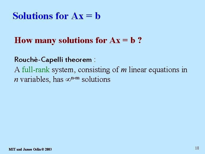
Solutions for Ax = b How many solutions for Ax = b ? Rouchè-Capelli theorem : A full-rank system, consisting of m linear equations in n variables, has ∞n-m solutions MIT and James Orlin © 2003 18

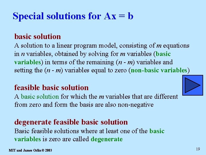
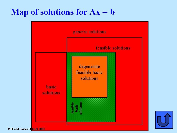
Special solutions for Ax = b basic solution A solution to a linear program model, consisting of m equations in n variables, obtained by solving for m variables (basic variables) in terms of the remaining (n - m) variables and setting the (n - m) variables equal to zero (non-basic variables) feasible basic solution A basic solution for which the m variables that are different from zero and form the basis are also non-negative degenerate feasible basic solution Basic feasible solutions where at least one of the basic variables is zero are called degenerate MIT and James Orlin © 2003 19

Map of solutions for Ax = b generic solutions feasible solutions degenerate feasible basic solutions MIT and James Orlin © 2003 20

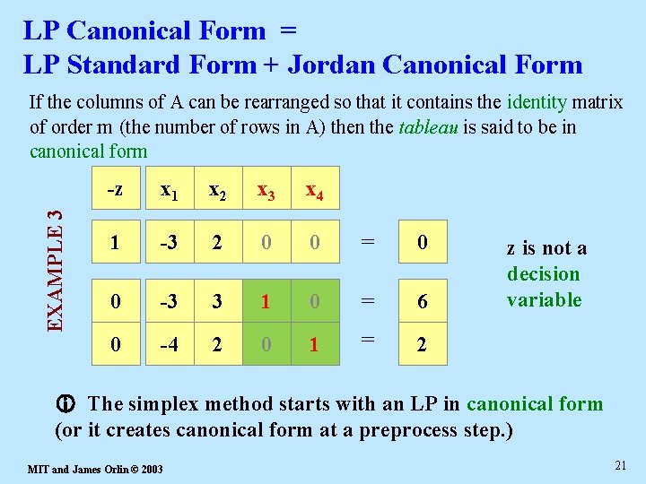
LP Canonical Form = LP Standard Form + Jordan Canonical Form EXAMPLE 3 If the columns of A can be rearranged so that it contains the identity matrix of order m (the number of rows in A) then the tableau is said to be in canonical form -z x 1 x 2 x 3 x 4 1 -3 2 0 0 = 0 0 -3 3 1 0 = 6 0 -4 2 0 1 = 2 z is not a decision variable The simplex method starts with an LP in canonical form (or it creates canonical form at a preprocess step. ) MIT and James Orlin © 2003 21

Overview of Lecture Getting an LP into standard form l Getting an LP into canonical form l The Simplex algoritm with ≤ constraints l MIT and James Orlin © 2003 22

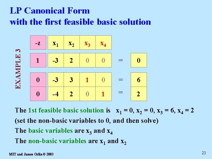
EXAMPLE 3 LP Canonical Form with the first feasible basic solution -z x 1 x 2 x 3 x 4 1 -3 2 0 0 = 0 0 -3 3 1 0 = 6 0 -4 2 0 1 = 2 The 1 st feasible basic solution is x 1 = 0, x 2 = 0, x 3 = 6, x 4 = 2 (set the non-basic variables to 0, and then solve) The basic variables are x 3 and x 4 The non-basic variables are x 1 and x 2 MIT and James Orlin © 2003 23

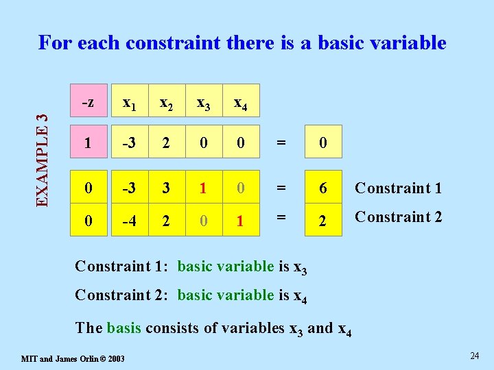
EXAMPLE 3 For each constraint there is a basic variable -z x 1 x 2 x 3 x 4 1 -3 2 0 0 = 0 0 -3 3 1 0 = 6 Constraint 1 0 -4 2 0 1 = 2 Constraint 1: basic variable is x 3 Constraint 2: basic variable is x 4 The basis consists of variables x 3 and x 4 MIT and James Orlin © 2003 24

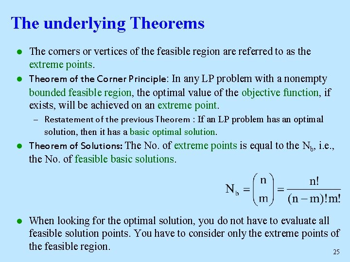
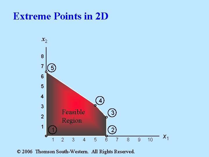
The underlying Theorems The corners or vertices of the feasible region are referred to as the extreme points. l Theorem of the Corner Principle: In any LP problem with a nonempty bounded feasible region, the optimal value of the objective function, if exists, will be achieved on an extreme point. l – Restatement of the previous Theorem : If an LP problem has an optimal solution, then it has a basic optimal solution. l Theorem of Solutions: The No. of extreme points is equal to the Nb, i. e. , the No. of feasible basic solutions. l When looking for the optimal solution, you do not have to evaluate all feasible solution points. You have to consider only the extreme points of the feasible region. 25

Extreme Points in 2 D x 2 8 7 5 6 5 4 4 3 Feasible Region 2 1 3 1 1 2 2 3 4 5 6 7 8 © 2006 Thomson South-Western. All Rights Reserved. 9 10 x 1

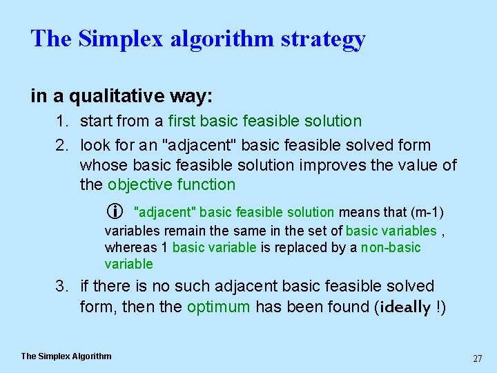
The Simplex algorithm strategy in a qualitative way: 1. start from a first basic feasible solution 2. look for an "adjacent" basic feasible solved form whose basic feasible solution improves the value of the objective function "adjacent" basic feasible solution means that (m-1) variables remain the same in the set of basic variables , whereas 1 basic variable is replaced by a non-basic variable 3. if there is no such adjacent basic feasible solved form, then the optimum has been found (ideally !) The Simplex Algorithm 27

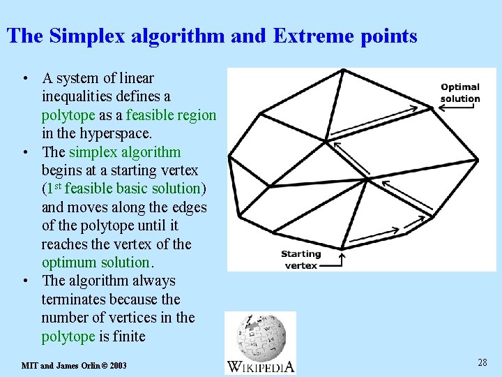
The Simplex algorithm and Extreme points • A system of linear inequalities defines a polytope as a feasible region in the hyperspace. • The simplex algorithm begins at a starting vertex (1 st feasible basic solution) and moves along the edges of the polytope until it reaches the vertex of the optimum solution. • The algorithm always terminates because the number of vertices in the polytope is finite MIT and James Orlin © 2003 28

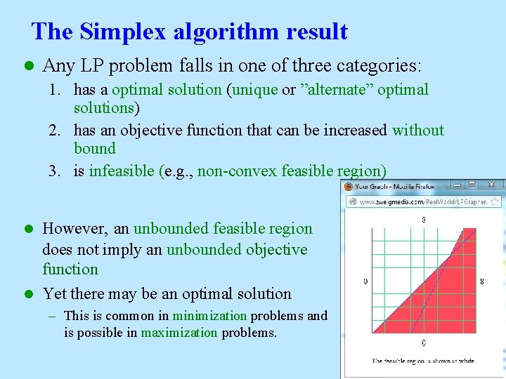
The Simplex algorithm result l Any LP problem falls in one of three categories: 1. has a optimal solution (unique or ”alternate” optimal solutions) 2. has an objective function that can be increased without bound 3. is infeasible (e. g. , non-convex feasible region) However, an unbounded feasible region does not imply an unbounded objective function l Yet there may be an optimal solution l – This is common in minimization problems and is possible in maximization problems.

Overview of Lecture Getting an LP into standard form l Getting an LP into canonical form l Optimality conditions l MIT and James Orlin © 2003 30

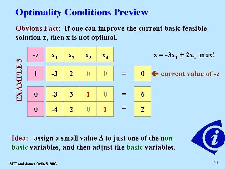
Optimality Conditions Preview EXAMPLE 3 Obvious Fact: If one can improve the current basic feasible solution x, then x is not optimal. -z x 1 x 2 x 3 x 4 1 -3 2 0 0 = 0 current value of -z 0 -3 3 1 0 = 6 0 -4 2 0 1 = 2 z = -3 x 1 + 2 x 2 max! Idea: assign a small value D to just one of the nonbasic variables, and then adjust the basic variables. MIT and James Orlin © 2003 31

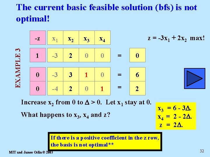
EXAMPLE 3 The current basic feasible solution (bfs) is not optimal! z = -3 x 1 + 2 x 2 max! -z x 1 x 2 x 3 x 4 1 -3 2 0 0 = 0 0 -3 3 1 0 = 6 0 -4 2 0 1 = 2 Increase x 2 from 0 to D > 0. Let x 1 stay at 0. What happens to x 3, x 4 and z? x 3 = 6 - 3 D. x 4 = 2 - 2 D. z = 2 D. If there is a positive coefficient in the z row, the basis is not optimal** MIT and James Orlin © 2003 32

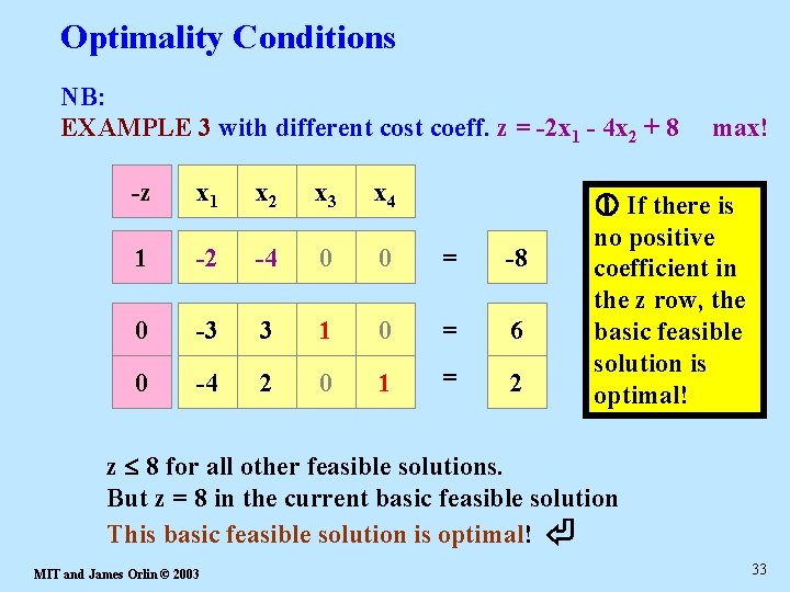
Optimality Conditions NB: EXAMPLE 3 with different cost coeff. z = -2 x 1 - 4 x 2 + 8 -z x 1 x 2 x 3 x 4 1 -2 -4 0 0 = -8 0 -3 3 1 0 = 6 0 -4 2 0 1 = 2 max! If there is no positive coefficient in the z row, the basic feasible solution is optimal! z 8 for all other feasible solutions. But z = 8 in the current basic feasible solution This basic feasible solution is optimal! ⏎ MIT and James Orlin © 2003 33

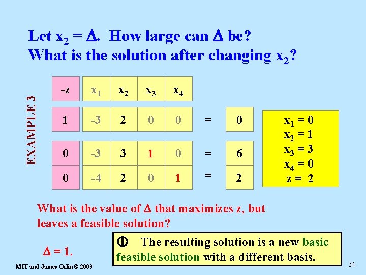
EXAMPLE 3 Let x 2 = D. How large can D be? What is the solution after changing x 2? -z x 1 x 2 x 3 x 4 1 -3 2 0 0 = 0 0 -3 3 1 0 = 6 0 -4 2 0 1 = 2 x 1 = 0 x 2 = D 1 x 3 =x 36=- 33 D. x 4 = x 42=-02 D. zz==2 D. 2 What is the value of D that maximizes z, but leaves a feasible solution? D = 1. MIT and James Orlin © 2003 The resulting solution is a new basic feasible solution with a different basis. 34

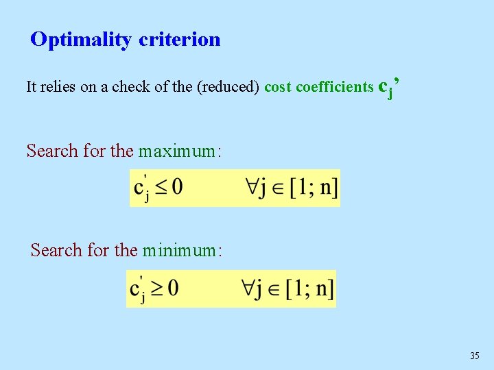
Optimality criterion It relies on a check of the (reduced) cost coefficients cj’ Search for the maximum: Search for the minimum: 35

Overview of Lecture Getting an LP into standard form l Getting an LP into canonical form l Optimality conditions l Improving a solution: a pivot l MIT and James Orlin © 2003 36

Improving a solution, a pivot l pivoting the algebraic manipulation of the Tableau l result of pivoting move one variable out of basic variables ( exit variable) and another one in ( entry variable) l adjacent solution the new basic feasible solution obtained just after one single pivoting operation on Tableau The Simplex Algorithm 11 November, 2002 37

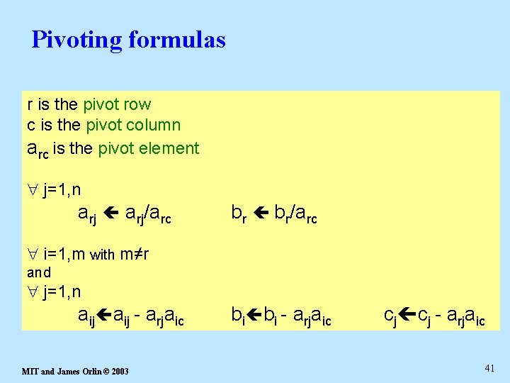
Text description of Pivoting • The geometrical operation of moving from a basic feasible solution to an adjacent basic feasible solution is implemented as a pivot operation. • First, a nonzero pivot element is selected in a non-basic column. • The row containing this element is multiplied by its reciprocal to change this element to 1, and then multiples of the row are added to the other rows to change the other entries in the column to 0. The result is that, if the pivot element is in row r, then the column becomes the r-th column of the identity matrix. • The variable for this column is now a basic variable, replacing the variable which corresponded to the r-th column of the identity matrix before the operation. • The variable corresponding to the pivot column enters the set of basic variables and is called the entering (entry) variable • The variable being replaced leaves the set of basic variables and is called the leaving (exit or departing) variable. • The tableau is still in canonical form, but with the set of basic variables changed by one element. MIT and James Orlin © 2003 38

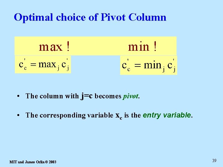
Optimal choice of Pivot Column max ! min ! • The column with j=c becomes pivot. • The corresponding variable xc is the entry variable. MIT and James Orlin © 2003 39

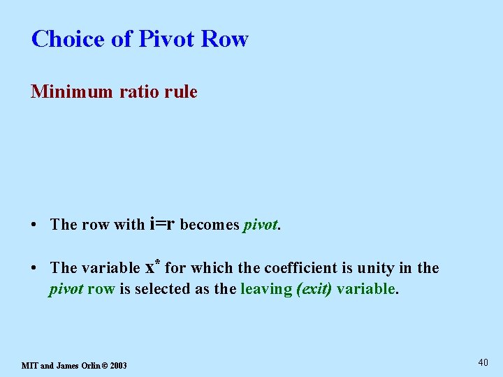
Choice of Pivot Row Minimum ratio rule • The row with i=r becomes pivot. • The variable x* for which the coefficient is unity in the pivot row is selected as the leaving (exit) variable. MIT and James Orlin © 2003 40

Pivoting formulas r is the pivot row c is the pivot column arc is the pivot element j=1, n arj/arc br br/arc i=1, m with m≠r and j=1, n aij - arjaic MIT and James Orlin © 2003 bi bi - arjaic cj cj - arjaic 41

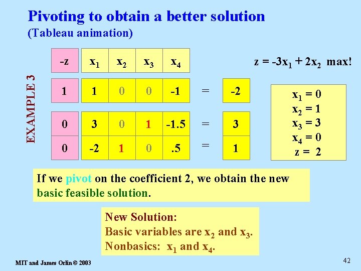
Pivoting to obtain a better solution EXAMPLE 3 (Tableau animation) -z x 1 x 2 x 3 x 4 1 -3 1 02 0 -1 0 = -2 0 0 -3 3 03 1 -1. 5 0 = 36 0 -4 -2 12 0 . 5 1 = 12 z = -3 x 1 + 2 x 2 max! x 1 = 0 x 2 = 1 x 3 = 3 x 4 = 0 z= 2 If we pivot on the coefficient 2, we obtain the new basic feasible solution. New Solution: Basic variables are x 2 and x 3. Nonbasics: x 1 and x 4. MIT and James Orlin © 2003 42

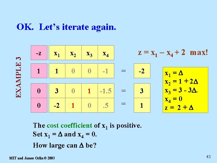
EXAMPLE 3 OK. Let’s iterate again. z = x 1 – x 4 + 2 max! -z x 1 x 2 x 3 x 4 1 1 0 0 -1 = -2 0 3 0 1 -1. 5 = 3 0 -2 1 0 . 5 = 1 x 1 = D x 2 = 1 + 2 D x 3 = 3 - 3 D. x 4 = 0 z= 2+D The cost coefficient of x 1 is positive. Set x 1 = D and x 4 = 0. How large can D be? MIT and James Orlin © 2003 43

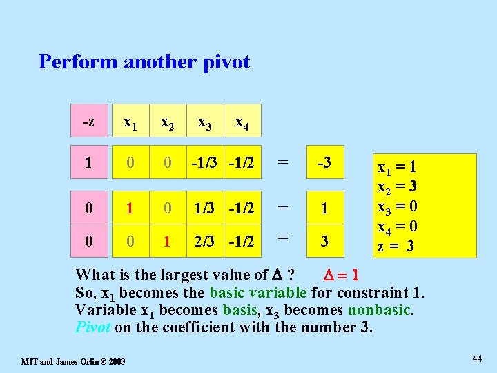
Perform another pivot -z x 1 x 2 x 3 x 4 1 01 0 -1/3 0 -1/2 -1 = -3 -2 0 31 0 1/3 1 -1/2 -1. 5 = 13 0 -2 0 1 2/3 0 -1/2. 5 = 31 x 1 = 1 D x 2 = 31 + 2 D x 3 = 03 - 3 D. x 4 = 0 z = 32 + D What is the largest value of D ? D = 1 So, x 1 becomes the basic variable for constraint 1. Variable x 1 becomes basis, x 3 becomes nonbasic. Pivot on the coefficient with the number 3. MIT and James Orlin © 2003 44

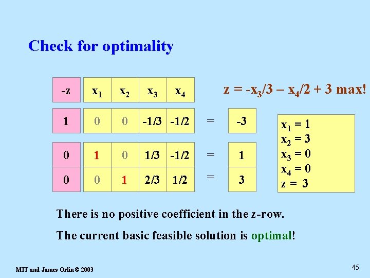
Check for optimality x 3 z = -x 3/3 – x 4/2 + 3 max! -z x 1 x 2 x 4 1 0 0 -1/3 -1/2 = -3 0 1/3 -1/2 = 1 0 0 1 2/3 1/2 = 3 x 1 = 1 D x 2 = 31 + 2 D x 3 = 03 - 3 D. x 4 = 0 z = 32 + D There is no positive coefficient in the z-row. The current basic feasible solution is optimal! MIT and James Orlin © 2003 45

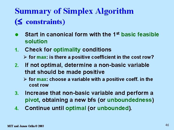
Summary of Simplex Algorithm ( constraints) l 1. Start in canonical form with the 1 st basic feasible solution Check for optimality conditions Ø for max: is there a positive coefficient in the cost row? 2. If not optimal, determine a non-basic variable that should be made positive Ø for max: choose a variable with a positive coeff. in the cost row 3. 4. Increase that non-basic variable and perform a pivot, obtaining a new bfs (or unboundedness) Continue until optimal (or unbounded). MIT and James Orlin © 2003 46