Chapter 3 The Laplace Transform 3 1 Definition

Chapter 3: The Laplace Transform 3. 1. Definition and Basic Properties 。 Objective of Laplace transform -- Convert differential into algebraic equations ○ Definition 3. 1: Laplace transform s. t. converges s, t : independent variables ＊ Representation: 1

。Example 3. 2: Consider 2

3

* Not every function has a Laplace transform. In general, can not converge 。Example 3. 1: 4

○ Definition 3. 2. : Piecewise continuity (PC) f is PC on if there are finite points s. t. and are finite i. e. , f is continuous on [a, b] except at finite points, at each of which f has finite one-sided limits 5

If f is PC on [0, k], then so is and exists 6

◎ Theorem 3. 2: Existence of f is PC on If Proof: 7

* Theorem 3. 2 is a sufficient but not a necessary condition. 8

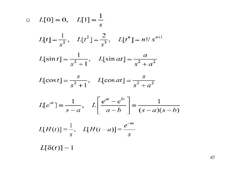
＊ There may be different functions whose Laplace transforms are the same e. g. , and have the same Laplace transform ○ Theorem 3. 3: Lerch’s Theorem ＊ Table 3. 1 lists Laplace transforms of functions 9

○ Theorem 3. 1: Laplace transform is linear Proof: ○ Definition 3. 3: . Inverse Laplace transform e. g. , ＊ Inverse Laplace transform is linear 10

3. 2 Solution of Initial Value Problems Using Laplace Transform ○ Theorem 3. 5: Laplace transform of f: continuous on : PC on [0, k] Then, ------(3. 1) 11

Proof: Let 12

○ Theorem 3. 6: Laplace transform of : PC on [0, k] for s > 0, j = 1, 2 … , n-1 13

。 Example 3. 3: From Table 3. 1, entries (5) and (8) 14

15

○ Laplace Transform of Integral From Eq. (3. 1), 16

3. 3. Shifting Theorems and Heaviside Function 3. 3. 1. The First Shifting Theorem ◎ Theorem 3. 7: ○ Example 3. 6: Given 17

○ Example 3. 8: 18

3. 3. 2. Heaviside Function and Pulses ○ f has a jump discontinuity at a, if exist and are finite but unequal ○ Definition 3. 4: Heaviside function 。 Shifting 19

。 Laplace transform of heaviside function 20

3. 3. 3 The Second Shifting Theorem ◎ Theorem 3. 8: Proof: 21

○ Example 3. 11: Rewrite 22

◎ The inverse version of the second shifting theorem ○ Example 3. 13: where rewritten as 23

24

25

3. 4. Convolution 26

◎ Theorem 3. 9: Convolution theorem Proof: 27

◎ Theorem 3. 10: ○ Exmaple 3. 18 ◎ Theorem 3. 11: Proof : 28

○ Example 3. 19: 29

3. 5 Impulses and Dirac Delta Function ○ Definition 3. 5: Pulse ○ Impulse: ○ Dirac delta function: A pulse of infinite magnitude over an infinitely short duration 30

○ Laplace transform of the delta function ◎ Filtering (Sampling) ○ Theorem 3. 12: f : integrable and continuous at a 31

Proof: 32

by Hospital’s rule ○ Example 3. 20: 33

3. 6 Laplace Transform Solution of Systems ○ Example 3. 22 Laplace transform Solve for 34

Partial fractions decomposition Inverse Laplace transform 35

3. 7. Differential Equations with Polynomial Coefficient ◎ Theorem 3. 13: Proof: ○ Corollary 3. 1: 36

○ Example 3. 25: Laplace transform 37

Find the integrating factor, Multiply (B) by the integrating factor 38

Inverse Laplace transform 39

○ Apply Laplace transform to algebraic expression for Y Apply Laplace transform to Differential equation for Y 40

◎ Theorem 3. 14: PC on [0, k], 41

○ Example 3. 26: Laplace transform ------(A) ------(B) 42

Finding an integrating factor, Multiply (B) by , 43

In order to have 44

Formulas: ○ Laplace Transform of Derivatives: ○ Laplace Transform of Integral: 45

○Shifting Theorems: ○ Convolution: Convolution Theorem: ○ 46