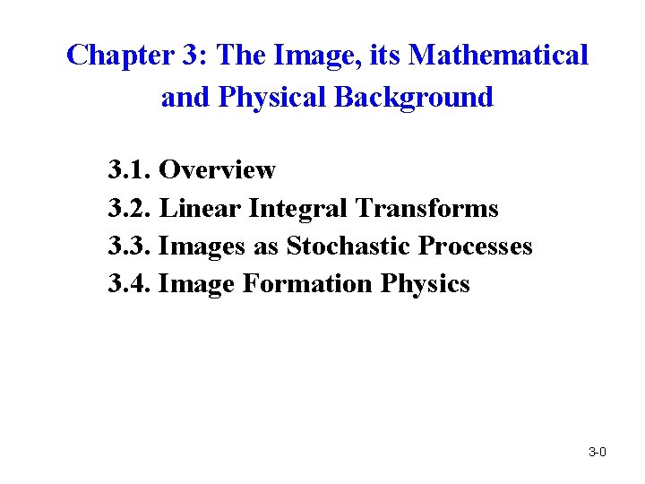
Chapter 3 The Image its Mathematical and Physical

Chapter 3: The Image, its Mathematical and Physical Background 3. 1. Overview 3. 2. Linear Integral Transforms 3. 3. Images as Stochastic Processes 3. 4. Image Formation Physics 3 -0

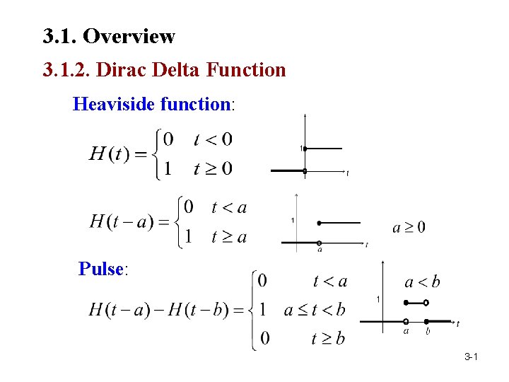
3. 1. Overview 3. 1. 2. Dirac Delta Function Heaviside function: Pulse: 3 -1

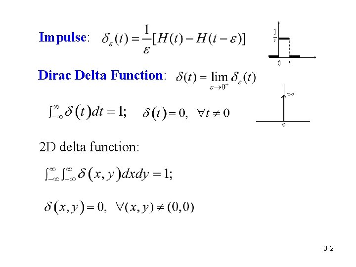
Impulse: Dirac Delta Function: 2 D delta function: 3 -2

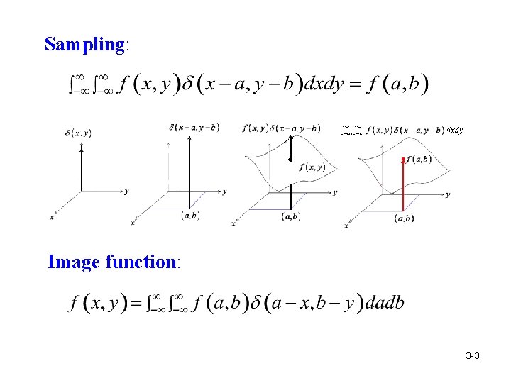
Sampling: Image function: 3 -3

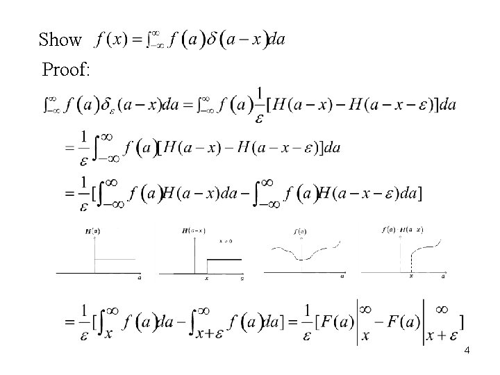
Show Proof: 4

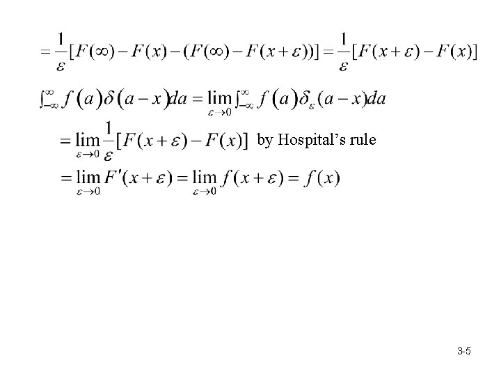
by Hospital’s rule 3 -5

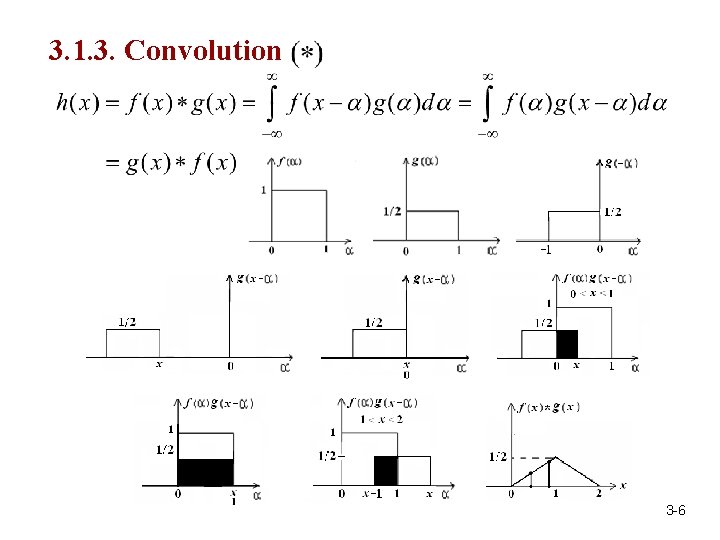
3. 1. 3. Convolution 3 -6

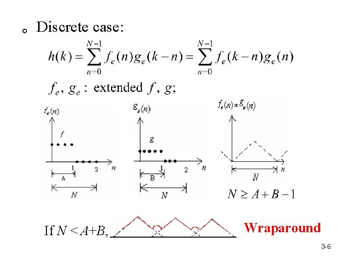
。Discrete case: If N < A+B, Wraparound 3 -6

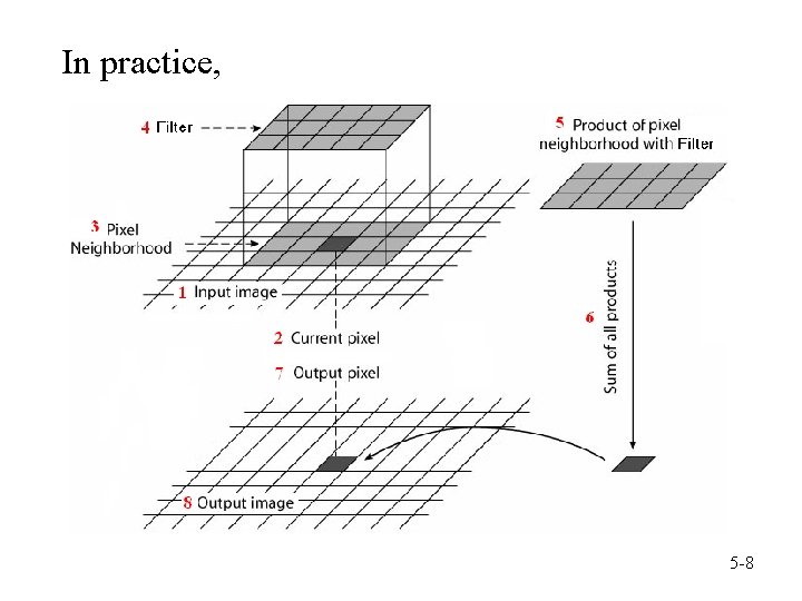
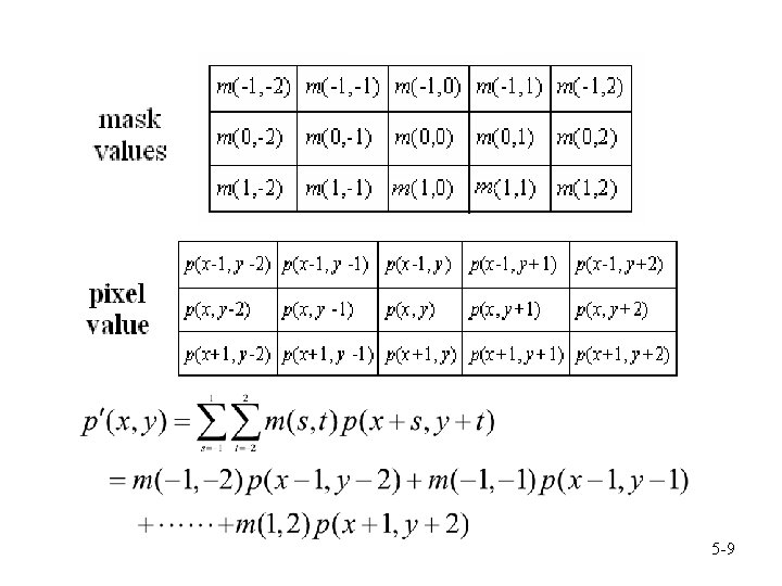
In practice, 5 -8

5 -9

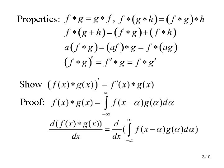
Properties: Show Proof: 3 -10

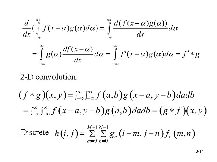
2 -D convolution: Discrete: 3 -11

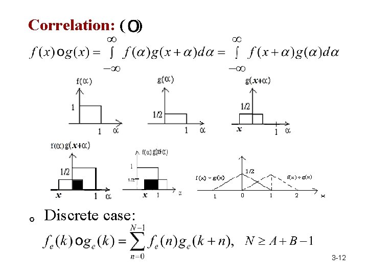
Correlation: ( ) 。Discrete case: 3 -12

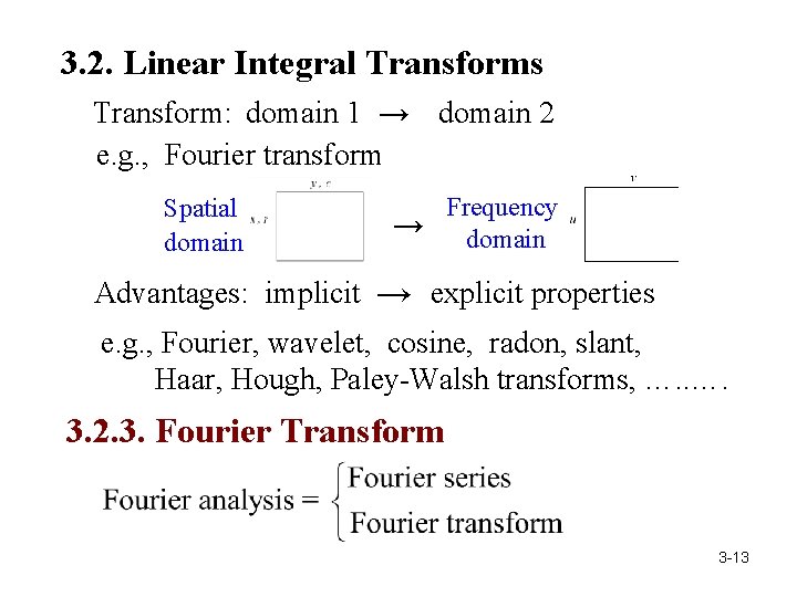
3. 2. Linear Integral Transforms Transform: domain 1 → domain 2 e. g. , Fourier transform Spatial domain Frequency → domain Advantages: implicit → explicit properties e. g. , Fourier, wavelet, cosine, radon, slant, Haar, Hough, Paley-Walsh transforms, …. 3. 2. 3. Fourier Transform 3 -13

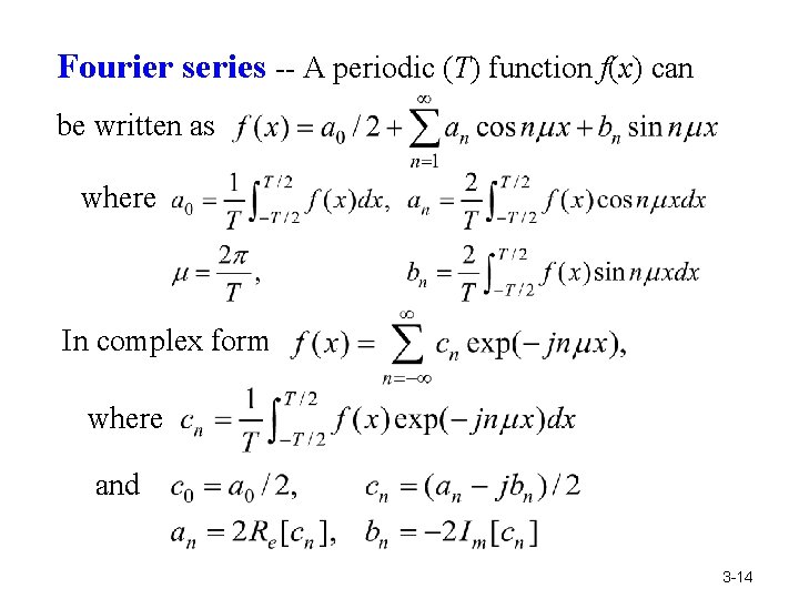
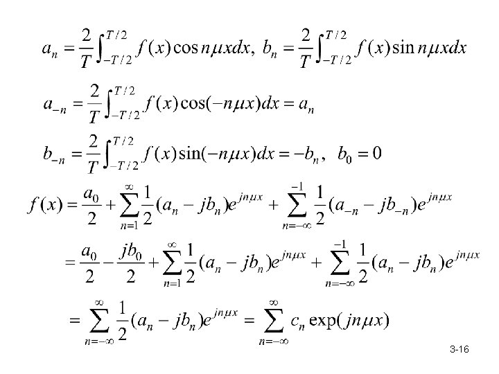
Fourier series -- A periodic (T) function f(x) can be written as where In complex form where and 3 -14

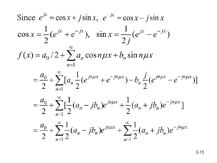
Since 3 -15

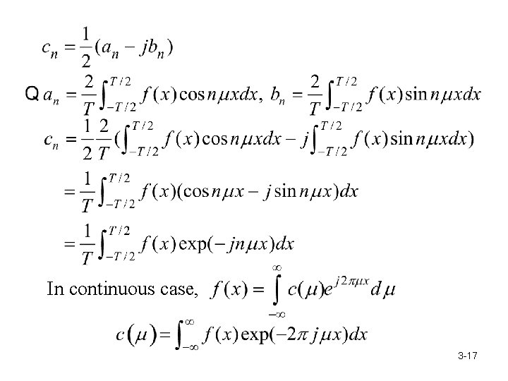
3 -16

In continuous case, 3 -17

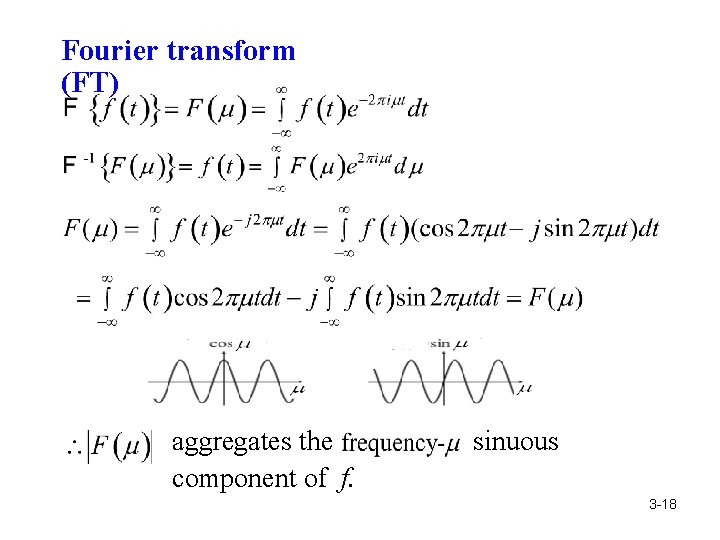
Fourier transform (FT) aggregates the component of f. sinuous 3 -18

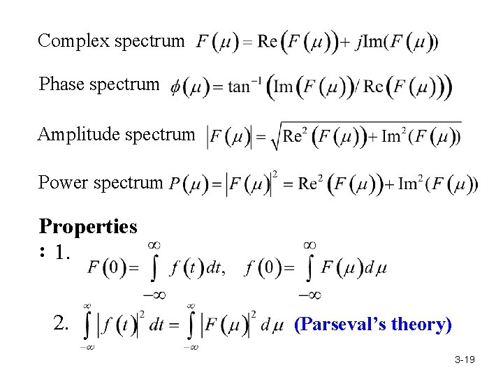
Complex spectrum Phase spectrum Amplitude spectrum Power spectrum Properties : 1. 2. (Parseval’s theory) 3 -19

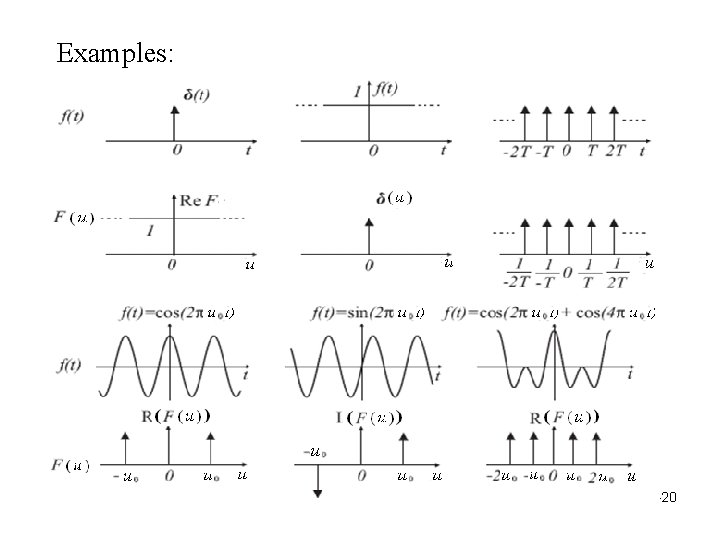
Examples: 3 -20

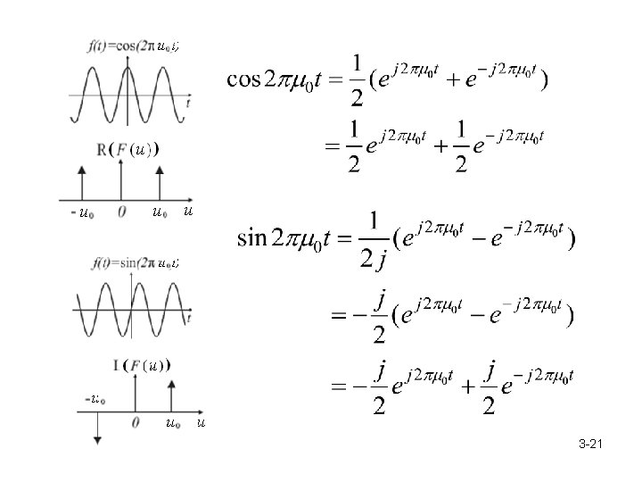
3 -21

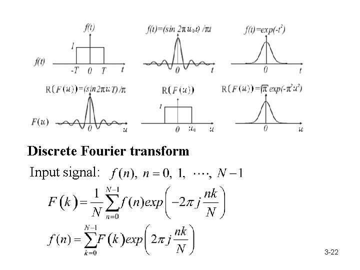
Discrete Fourier transform Input signal: 3 -22

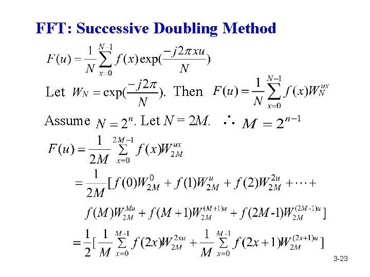
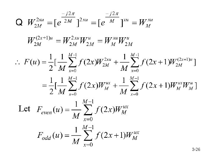
FFT: Successive Doubling Method Let Assume Then. Let N = 2 M. ∴ 3 -23

Let 3 -26

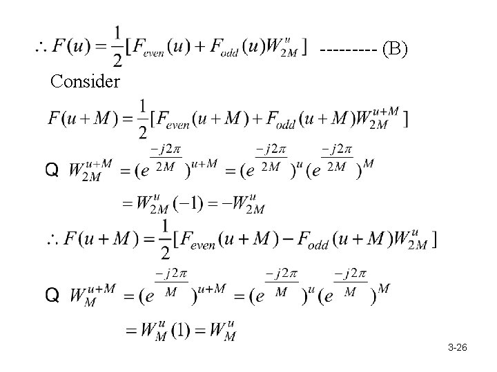
----- (B) Consider 3 -26

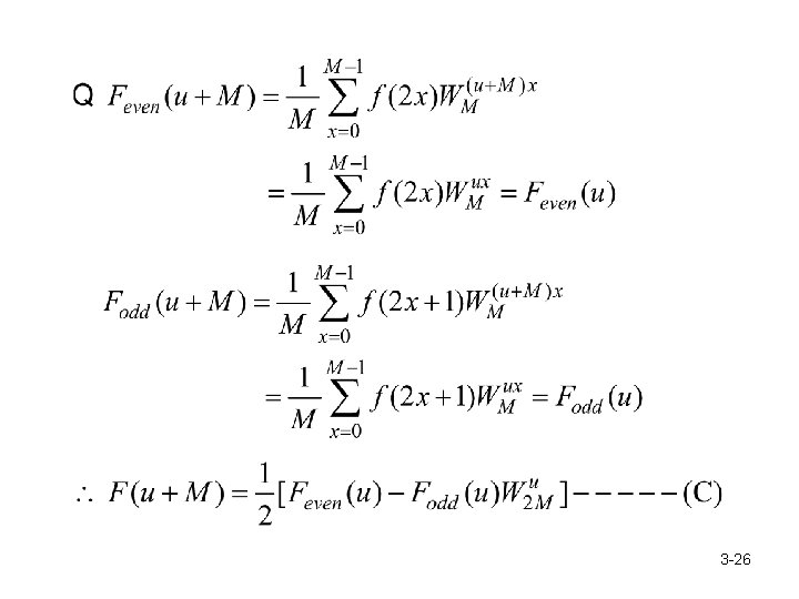
3 -26

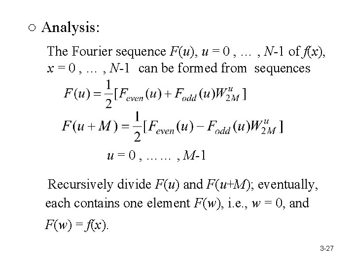
○ Analysis: The Fourier sequence F(u), u = 0 , … , N-1 of f(x), x = 0 , … , N-1 can be formed from sequences u = 0 , …… , M-1 Recursively divide F(u) and F(u+M); eventually, each contains one element F(w), i. e. , w = 0, and F(w) = f(x). 3 -27

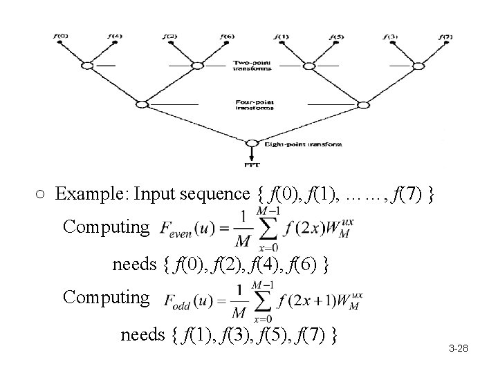
○ Example: Input sequence { f(0), f(1), ……, f(7) } Computing needs { f(0), f(2), f(4), f(6) } Computing needs { f(1), f(3), f(5), f(7) } 3 -28

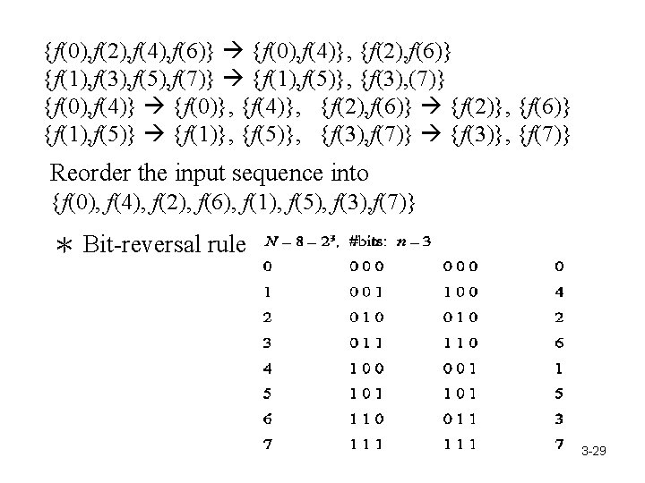
{f(0), f(2), f(4), f(6)} {f(0), f(4)}, {f(2), f(6)} {f(1), f(3), f(5), f(7)} {f(1), f(5)}, {f(3), (7)} {f(0), f(4)} {f(0)}, {f(4)}, {f(2), f(6)} {f(2)}, {f(6)} {f(1), f(5)} {f(1)}, {f(5)}, {f(3), f(7)} {f(3)}, {f(7)} Reorder the input sequence into {f(0), f(4), f(2), f(6), f(1), f(5), f(3), f(7)} ＊ Bit-reversal rule 3 -29

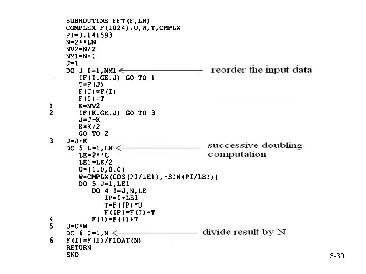
3 -30

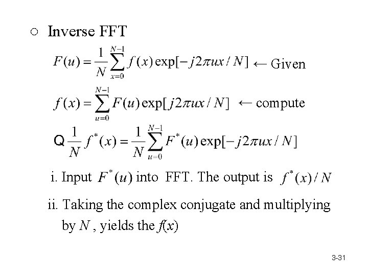
○ Inverse FFT ← Given ← compute i. Input into FFT. The output is ii. Taking the complex conjugate and multiplying by N , yields the f(x) 3 -31

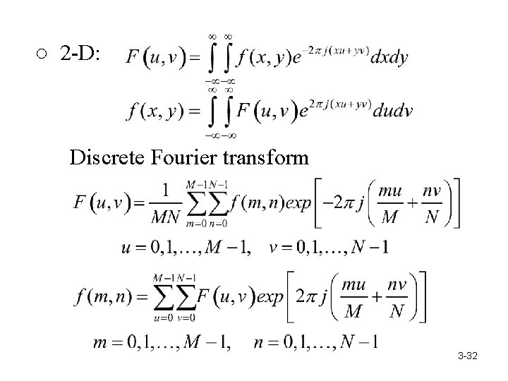
○ 2 -D: Discrete Fourier transform 3 -32

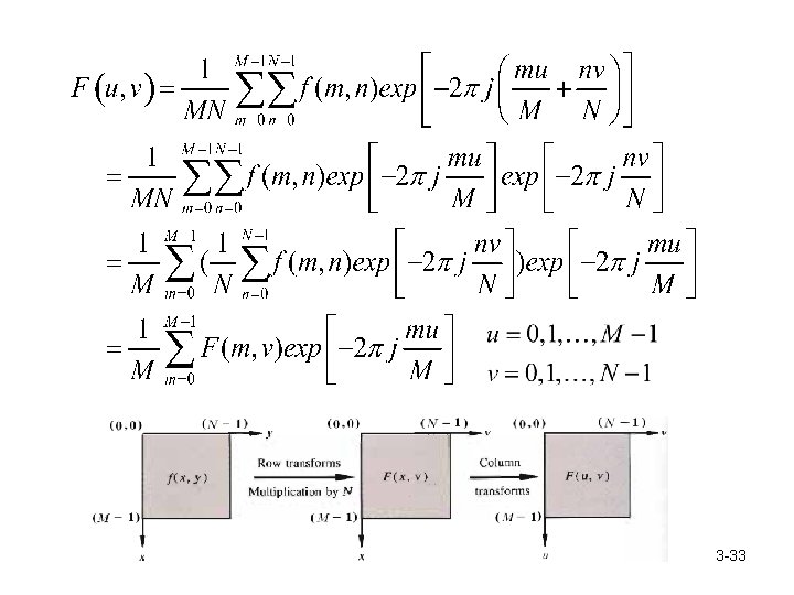
3 -33

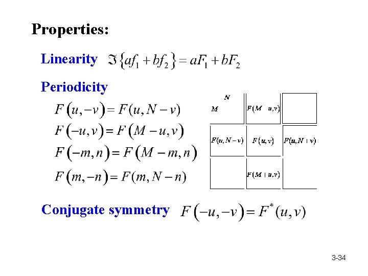
Properties: Linearity Periodicity Conjugate symmetry 3 -34

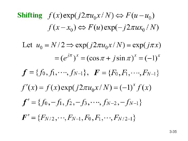
Shifting 3 -35

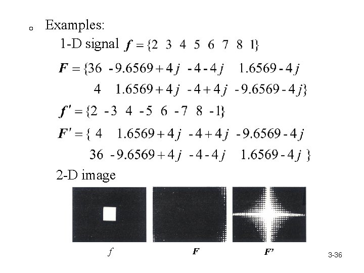
。 Examples: 1 -D signal 2 -D image f F F’ 3 -36

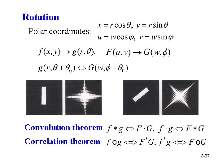
Rotation Polar coordinates: Convolution theorem Correlation theorem 3 -37

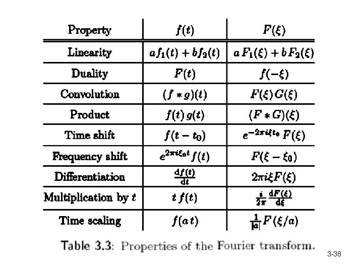
3 -38

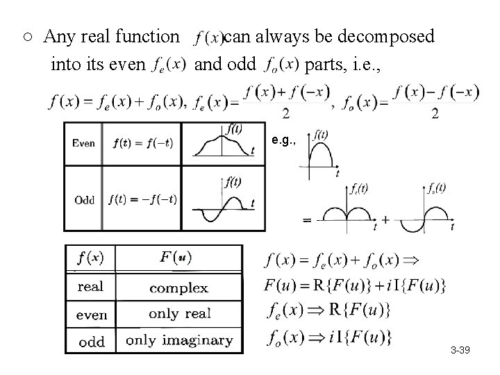
○ Any real function can always be decomposed into its even and odd parts, i. e. , e. g. , 3 -39

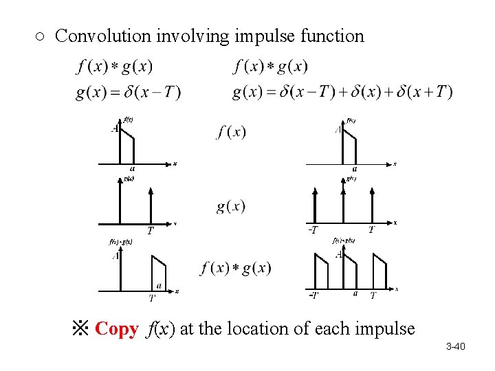
○ Convolution involving impulse function ※ Copy f(x) at the location of each impulse 3 -40

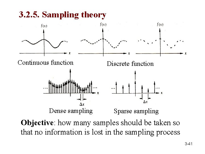
3. 2. 5. Sampling theory Continuous function Dense sampling Discrete function Sparse sampling Objective: how many samples should be taken so that no information is lost in the sampling process 3 -41

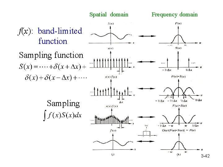
Spatial domain Frequency domain f(x): band-limited function Sampling 3 -42

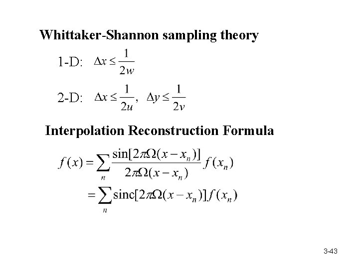
Whittaker-Shannon sampling theory 1 -D: 2 -D: Interpolation Reconstruction Formula 3 -43

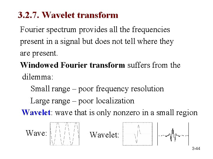
3. 2. 7. Wavelet transform Fourier spectrum provides all the frequencies present in a signal but does not tell where they are present. Windowed Fourier transform suffers from the dilemma: Small range – poor frequency resolution Large range – poor localization Wavelet: wave that is only nonzero in a small region Wave: Wavelet: 3 -44

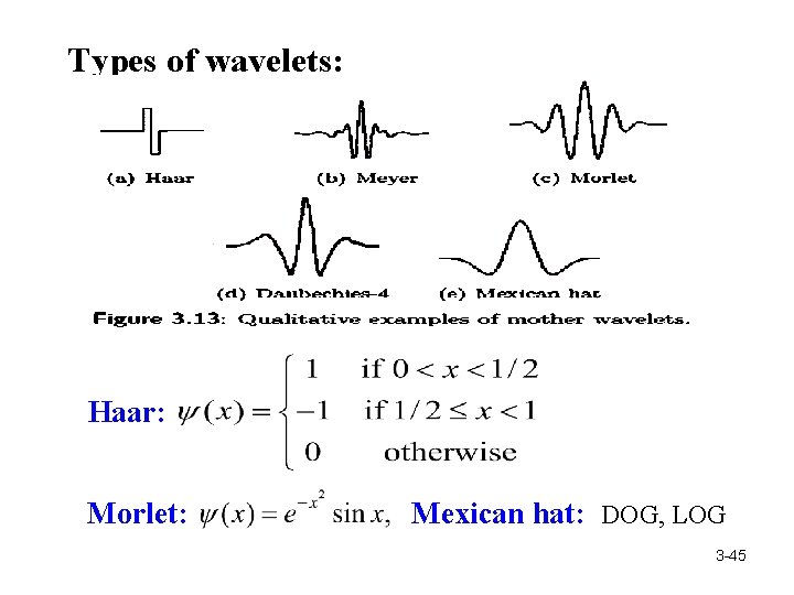
Types of wavelets: Haar: Morlet: Mexican hat: DOG, LOG 3 -45

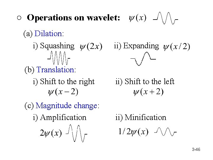
○ Operations on wavelet: (a) Dilation: i) Squashing ii) Expanding (b) Translation: i) Shift to the right ii) Shift to the left (c) Magnitude change: i) Amplification ii) Minification 3 -46

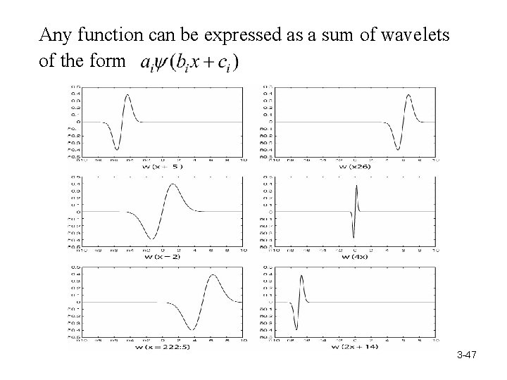
Any function can be expressed as a sum of wavelets of the form 3 -47

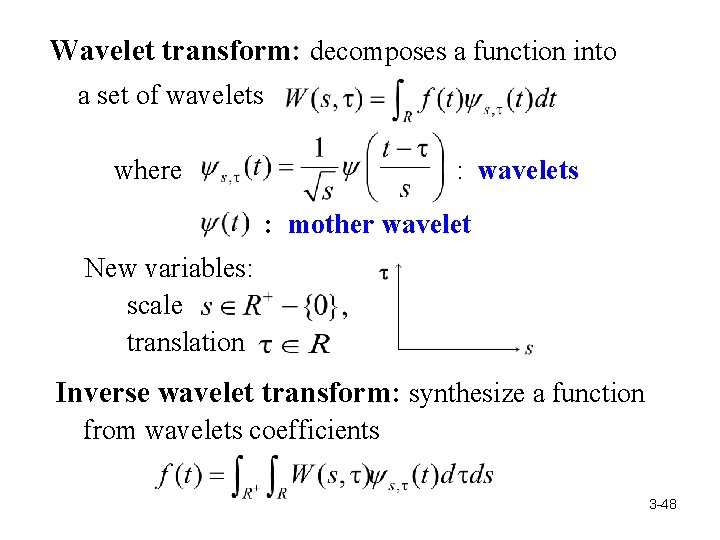
Wavelet transform: decomposes a function into a set of wavelets where : wavelets : mother wavelet New variables: scale translation Inverse wavelet transform: synthesize a function from wavelets coefficients 3 -48

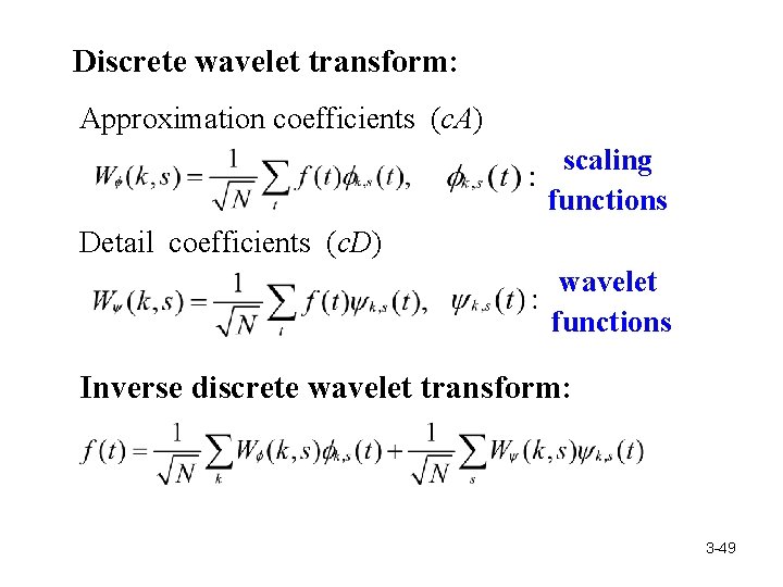
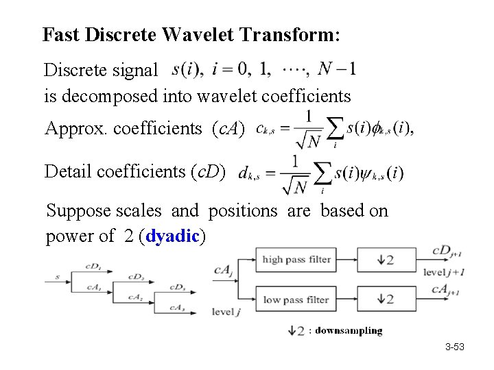
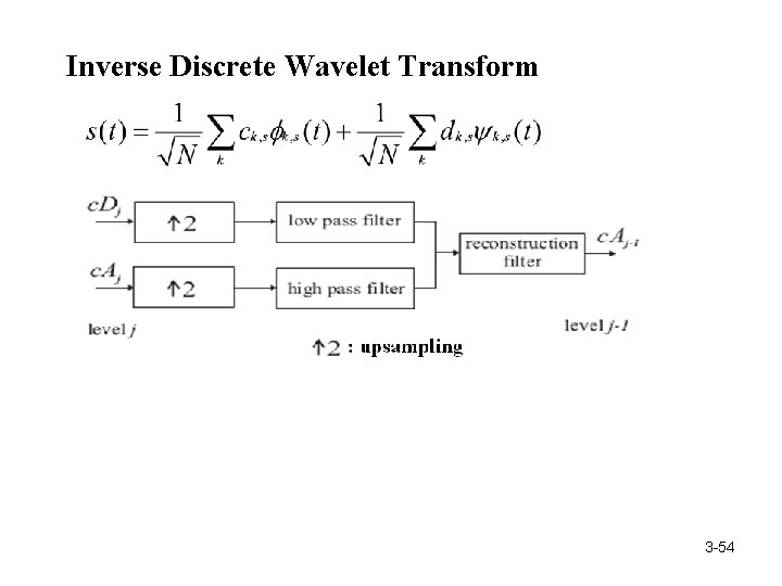
Discrete wavelet transform: Approximation coefficients (c. A) scaling functions Detail coefficients (c. D) wavelet functions Inverse discrete wavelet transform: 3 -49

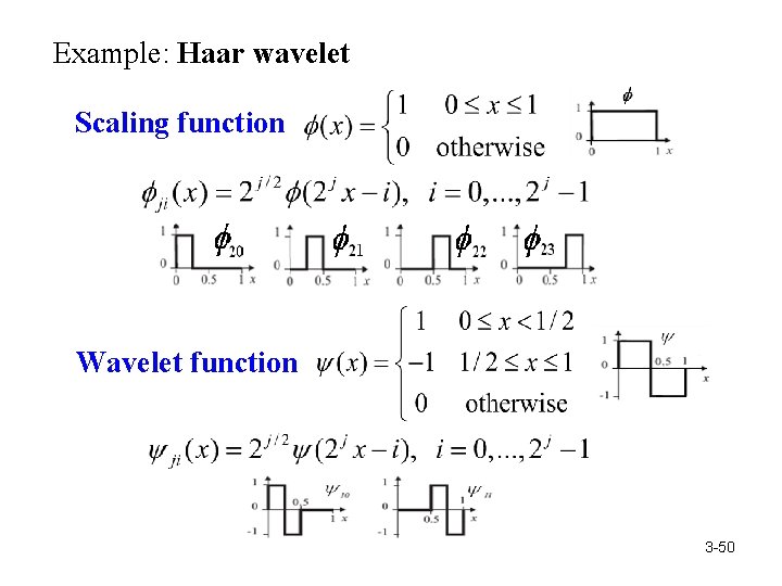
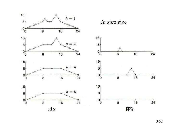
Example: Haar wavelet Scaling function Wavelet function 3 -50

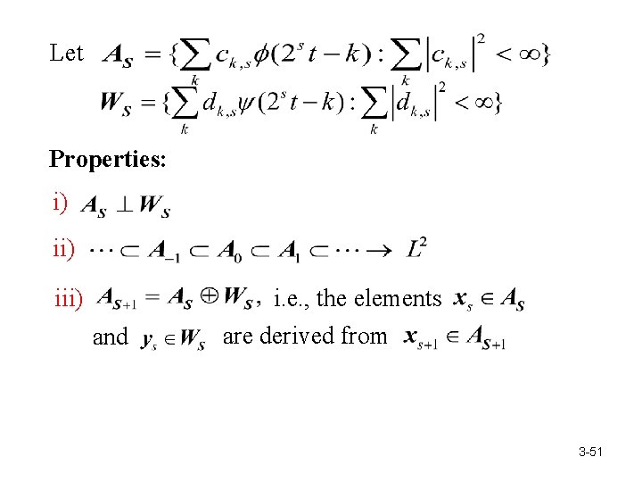
Let Properties: i) iii) i. e. , the elements and are derived from 3 -51

h: step size 3 -52

Fast Discrete Wavelet Transform: Discrete signal is decomposed into wavelet coefficients Approx. coefficients (c. A) Detail coefficients (c. D) Suppose scales and positions are based on power of 2 (dyadic) 3 -53

Inverse Discrete Wavelet Transform 3 -54

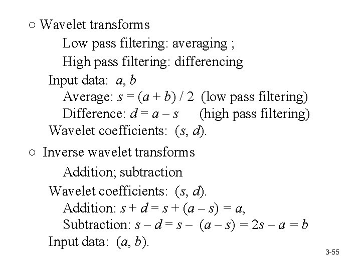
○ Wavelet transforms Low pass filtering: averaging ; High pass filtering: differencing Input data: a, b Average: s = (a + b) / 2 (low pass filtering) Difference: d = a – s (high pass filtering) Wavelet coefficients: (s, d). ○ Inverse wavelet transforms Addition; subtraction Wavelet coefficients: (s, d). Addition: s + d = s + (a – s) = a, Subtraction: s – d = s – (a – s) = 2 s – a = b Input data: (a, b). 3 -55

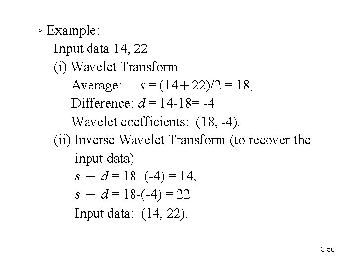
。Example: Input data 14, 22 (i) Wavelet Transform Average: s = (14＋22)/2 = 18, Difference: d = 14 -18= -4 Wavelet coefficients: (18, -4). (ii) Inverse Wavelet Transform (to recover the input data) s ＋ d = 18+(-4) = 14, s － d = 18 -(-4) = 22 Input data: (14, 22). 3 -56

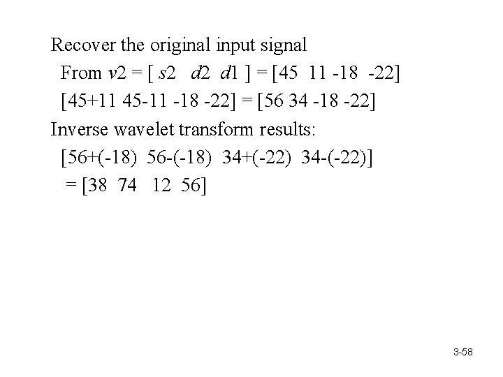
。Example: Input vector: v = [38 74 12 56] Average vector: s 1 = [(38+74)/2 (12+56)/2] = [56 34] Difference vector: d 1 = [38 -56 12 -34] = [-18 -22] Wavelet transform at 1 scale: v 1 = [ s 1 d 1 ] = [56 34 -18 -22] Average vector: s 2 = [(56+34)/2] = [45] Difference vector: d 2 = [56 -45] = [11] Wavelet transform at 2 scale: v 2 = [ s 2 d 1 ] = [45 11 -18 -22] 3 -57

Recover the original input signal From v 2 = [ s 2 d 1 ] = [45 11 -18 -22] [45+11 45 -11 -18 -22] = [56 34 -18 -22] Inverse wavelet transform results: [56+(-18) 56 -(-18) 34+(-22) 34 -(-22)] = [38 74 12 56] 3 -58

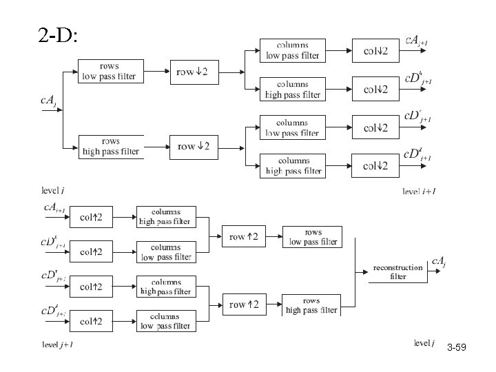
2 -D: 3 -59

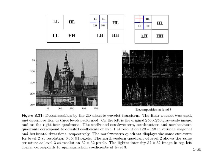
3 -60

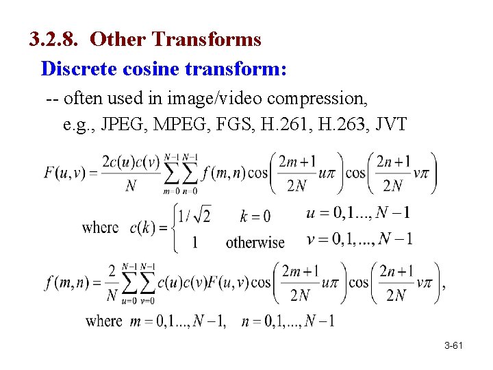
3. 2. 8. Other Transforms Discrete cosine transform: -- often used in image/video compression, e. g. , JPEG, MPEG, FGS, H. 261, H. 263, JVT 3 -61

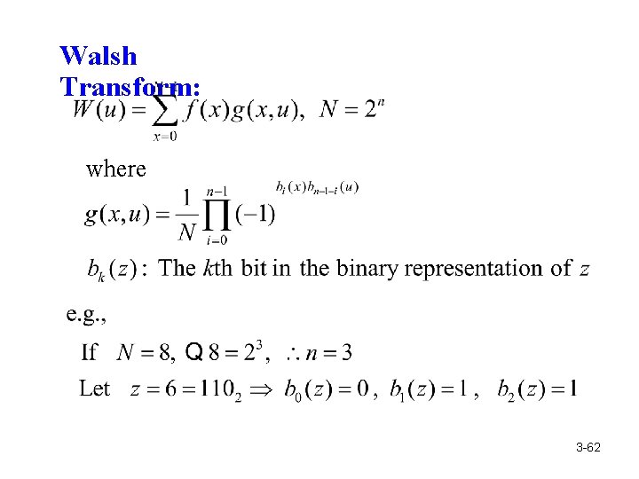
Walsh Transform: where 3 -62

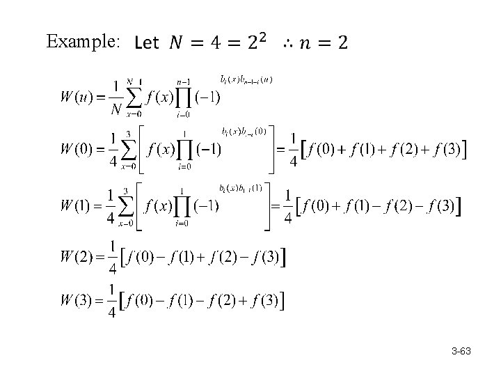
Example: 3 -63

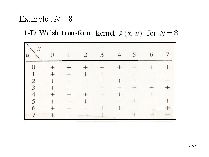
Example : N = 8 3 -64

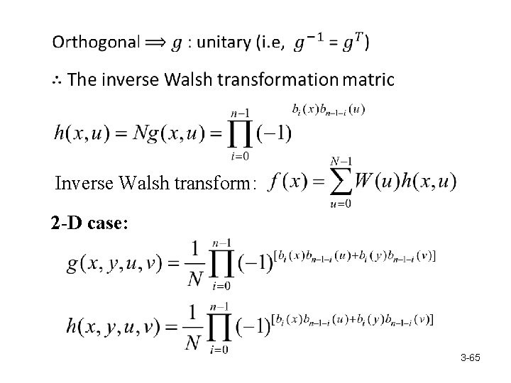
Inverse Walsh transform: 2 -D case: 3 -65

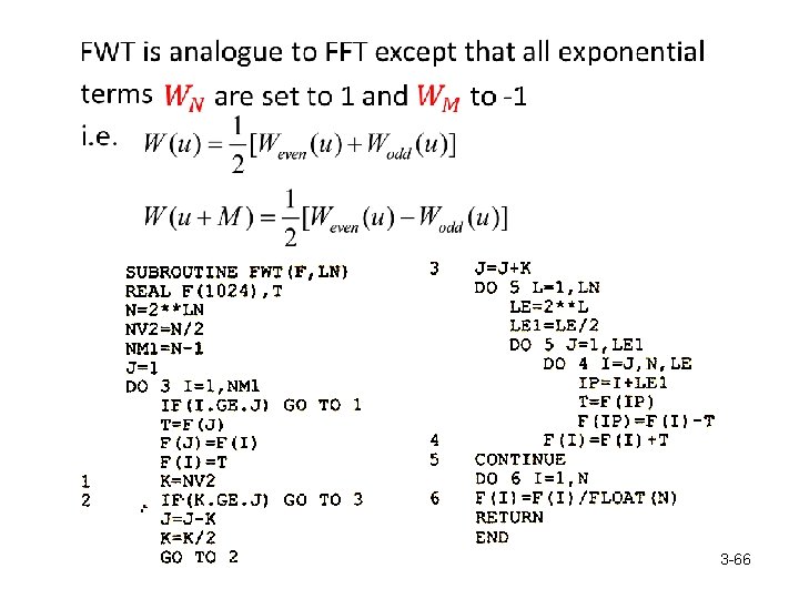
3 -66

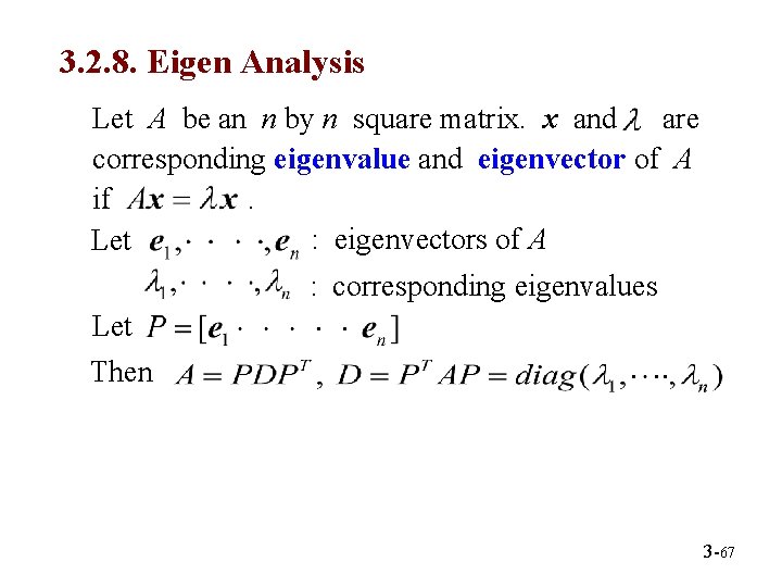
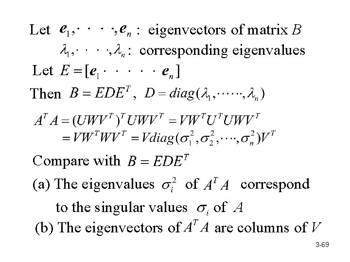
3. 2. 8. Eigen Analysis Let A be an n by n square matrix. x and are corresponding eigenvalue and eigenvector of A if. : eigenvectors of A Let : corresponding eigenvalues Let Then 3 -67

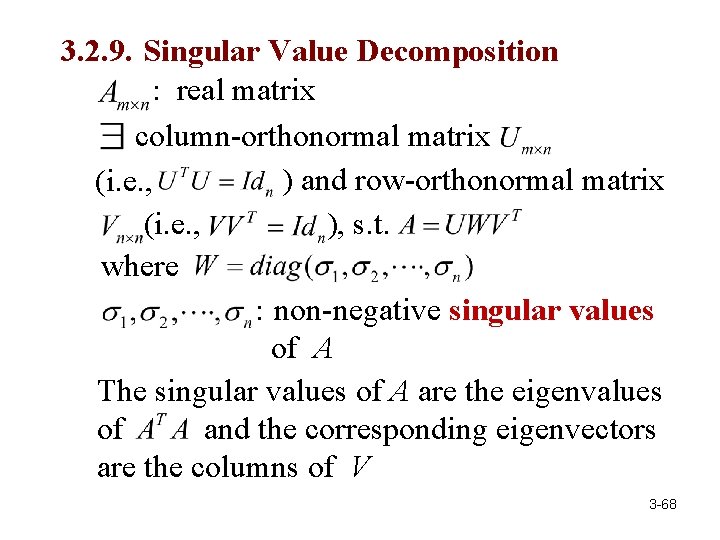
3. 2. 9. Singular Value Decomposition : real matrix column-orthonormal matrix ) and row-orthonormal matrix (i. e. , ), s. t. (i. e. , where : non-negative singular values of A The singular values of A are the eigenvalues of and the corresponding eigenvectors are the columns of V 3 -68

Let : eigenvectors of matrix B : corresponding eigenvalues Let Then Compare with (a) The eigenvalues of correspond to the singular values of A (b) The eigenvectors of are columns of V 3 -69

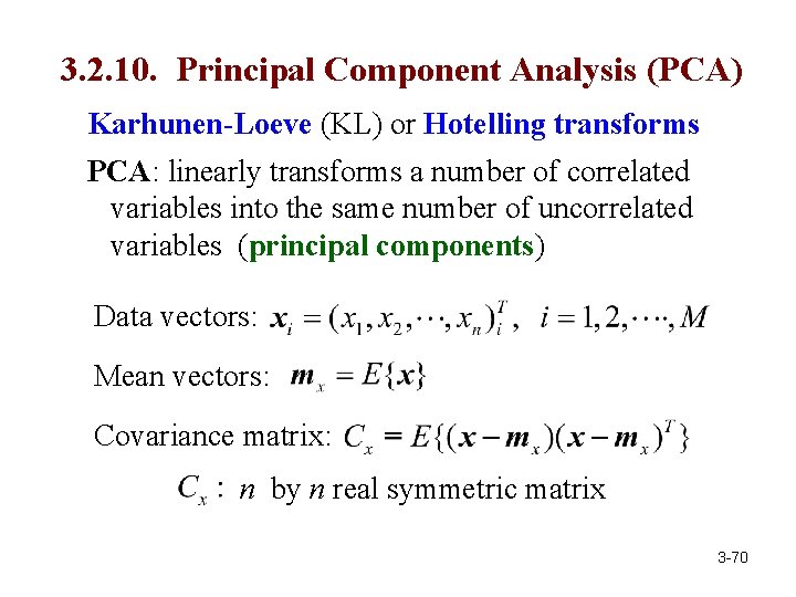
3. 2. 10. Principal Component Analysis (PCA) Karhunen-Loeve (KL) or Hotelling transforms PCA: linearly transforms a number of correlated variables into the same number of uncorrelated variables (principal components) Data vectors: Mean vectors: Covariance matrix: n by n real symmetric matrix 3 -70

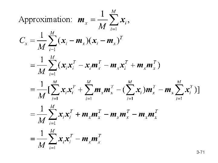
Approximation: 3 -71 71

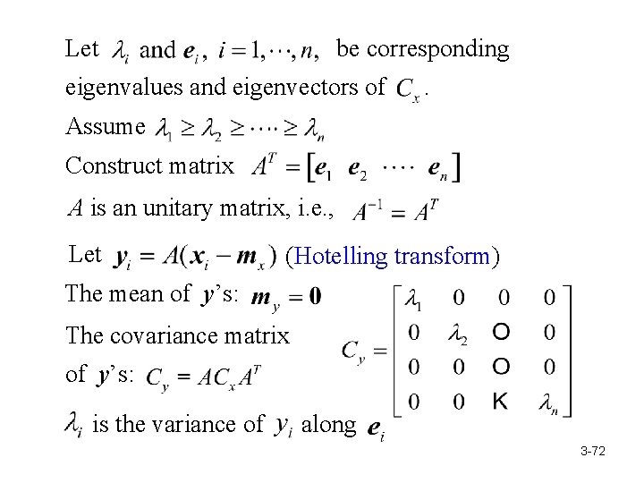
Let be corresponding eigenvalues and eigenvectors of . Assume Construct matrix A is an unitary matrix, i. e. , Let (Hotelling transform) The mean of y’s: The covariance matrix of y’s: is the variance of along 3 -72 72

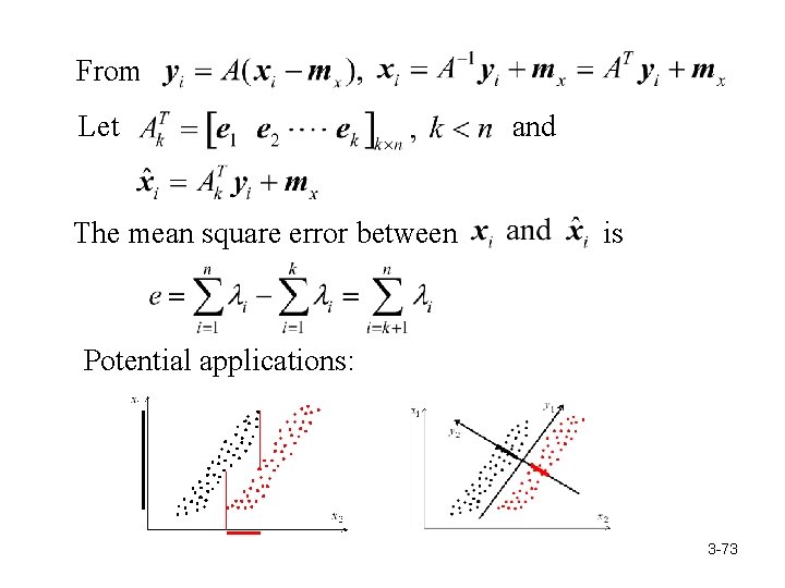
From Let The mean square error between and is Potential applications: 3 -73

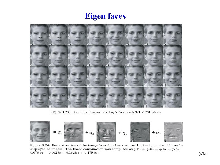
Eigen faces 3 -74 74